Weighted Graph

Weighted directed graph

Adjacency matrix representation in Python

# Each tuple (u,v,d) in list is representing the edge from u to v with weight d
dedges = [(0,1,10),(0,2,80),(1,2,6),(1,4,20),(2,3,70),(4,5,50),(4,6,5),(5,6,10)]
size = 7
import numpy as np
W = np.zeros(shape=(size,size,2))
for (i,j,w) in dedges:
    W[i,j,0] = 1
    W[i,j,1] = w
print(W)

 

Adjacency list representation in Python

dedges = [(0,1,10),(0,2,80),(1,2,6),(1,4,20),(2,3,70),(4,5,50),(4,6,5),(5,6,10)]
size = 7
WL = {}
for i in range(size):
    WL[i] = []
for (i,j,d) in dedges:
    WL[i].append((j,d))
print(WL)

 

 

Weighted undirected graph

Adjacency matrix representation in Python

dedges = [(0,1,10),(0,2,80),(1,2,6),(1,4,20),(2,3,70),(4,5,50),(4,6,5),(5,6,10)]
# Each edge represented by two entry in data structure ((u,v,d) and (v,u,d) for undirected graph
edges = dedges + [(j,i,w) for (i,j,w) in dedges]
size = 7
import numpy as np
W = np.zeros(shape=(size,size,2))
for (i,j,w) in edges:
    W[i,j,0] = 1
    W[i,j,1] = w
print(W)

 

Adjacency list representation in Python

dedges = [(0,1,10),(0,2,80),(1,2,6),(1,4,20),(2,3,70),(4,5,50),(4,6,5),(5,6,10)]
edges = dedges + [(j,i,w) for (i,j,w) in dedges]
size = 7
WL = {}
for i in range(size):
    WL[i] = []
for (i,j,d) in edges:
    WL[i].append((j,d))
print(WL)

 

---

 

Shortest Path

Single source shortest path algorithm

Find shortest paths from a source vertex to every other vertex.

• Dijkstra's Algorithm
• Bellman Ford algorithm

Dijkstra's Algorithm

Dijkstra's algorithm is a popular algorithm for finding the shortest path between two vertices in a weighted graph. Some of its important properties and points are:

1. Single-source shortest path: Dijkstra's algorithm finds the shortest path from a single source vertex to all other vertices in the graph.
2. Weighted graph: Dijkstra's algorithm only works on weighted graphs, where each edge has a weight or cost associated with it.
3. Non-negative weights: Dijkstra's algorithm can only be used on graphs with non-negative edge weights. If the graph contains negative weights, Bellman-Ford algorithm is a better choice.
4. Greedy algorithm: Dijkstra's algorithm is a greedy algorithm that selects the vertex with the smallest distance from the starting vertex and explores its neighbors. This process is repeated until the shortest path to all vertices is found.
5. Optimal substructure: Dijkstra's algorithm relies on the optimal substructure property, which means that the optimal solution to a problem can be obtained by combining the optimal solutions to its subproblems.
6. Can handle disconnected graphs: Dijkstra's algorithm can handle disconnected graphs, but it will only find the shortest path for the connected component containing the source vertex.

 

Algorithm Steps

Here are the steps for Dijkstra's algorithm for finding the single source shortest path:

1. Create a table to store the distances from the source vertex to each vertex in the graph. Initialize the source vertex with a distance of 0 and all other vertices with infinity. Also create a set of unvisited vertices and mark all vertices as unvisited.
2. While the set of unvisited vertices is not empty, do the following:
3. Select the unvisited vertex with the smallest distance from the source vertex. This vertex is now considered visited.
4. For each neighbor of the visited vertex that is still unvisited, calculate the distance to that neighbor by adding the weight of the edge between the visited vertex and the neighbor to the distance of the visited vertex. If this distance is smaller than the distance currently stored for the neighbor in the table, update the table with the new distance.
5. After updating the distances for all neighbors, mark the visited vertex as visited.
6. Repeat steps 3 to 5 until all vertices have been visited or the destination vertex has been visited.
7. Once the algorithm has visited all vertices, the table will contain the shortest distances from the source vertex to each vertex in the graph.
8. To find the shortest path from the source vertex to a destination vertex, backtrack from the destination vertex to the source vertex by following the path with the smallest distance at each step. This will give you the shortest path from the source vertex to the destination vertex.

 

Working Visualization

Open Visualization

Select Dijkstra(s) form left bottom menu

 

For given graph

 

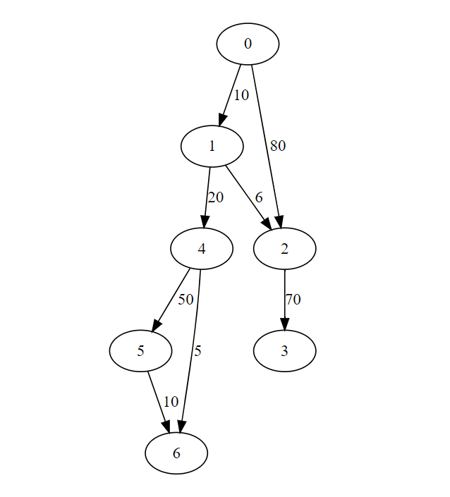
Implementation Dijkstra's For Adjacency matrix

def dijkstra(WMat,s):
    #Initialization
    (rows,cols,x) = WMat.shape
    infinity = np.max(WMat)*rows+1
    (visited,distance) = ({},{})
    for v in range(rows):
        (visited[v],distance[v]) = (False,infinity)        
    distance[s] = 0
    
    # Computing shortest distance for each vertex from source
    for u in range(rows):
        # Find minimum distance value on vertices which are not visited
        min_dist = min([distance[v] for v in range(rows) if not visited[v]])
        
        # Find vertices which have minimum distance value min_dist
        nextv_list = [v for v in range(rows)if (not visited[v]) and distance[v] == min_dist]
        
        # Select minimum level vertex which have minimum distance value min_dist and mark visited
        nextv = min(nextv_list)
        visited[nextv] = True
        
        # Check for each adjacent of nextv vertex which is not visited
        for v in range(cols):            
            if WMat[nextv,v,0] == 1 and (not visited[v]):
                #If distance of v through nextv is smaller than the current distance on v, then update
                if distance[nextv] + WMat[nextv,v,1] < distance[v]:
                    distance[v] = distance[nextv] + WMat[nextv,v,1]
    return(distance)



dedges = [(0,1,10),(0,2,80),(1,2,6),(1,4,20),(2,3,70),(4,5,50),(4,6,5),(5,6,10)]
size = 7
import numpy as np
W = np.zeros(shape=(size,size,2))
for (i,j,w) in dedges:
    W[i,j,0] = 1
    W[i,j,1] = w
print(dijkstra(W,0))

Output

{0: 0, 1: 10.0, 2: 16.0, 3: 86.0, 4: 30.0, 5: 80.0, 6: 35.0}

Complexity

$O(V^2 )$

 

Implementation Dijkstra's For Adjacency List

def dijkstralist(WList,s):
    #Initialization
    infinity = 1 + len(WList.keys())*max([d for u in WList.keys() for (v,d) in WList[u]])
    (visited,distance) = ({},{})
    for v in WList.keys():
        (visited[v],distance[v]) = (False,infinity)        
    distance[s] = 0
    
    # Computing shortest distance for each vertex from source
    for u in WList.keys():
        # Find minimum distance value on vertices which are not visited
        min_dist = min([distance[v] for v in WList.keys() if not visited[v]])
        
        # Find vertices which have minimum distance value min_dist
        nextv_list = [v for v in WList.keys() if (not visited[v]) and distance[v] == min_dist]

        # Select minimum level vertex which have minimum distance value min_dist and mark visited
        nextv = min(nextv_list)
        visited[nextv] = True
        
        # Check for each adjacent of nextv vertex which is not visited
        for (v,d) in WList[nextv]:
            if not visited[v]:
                # If distance of v through nextv is smaller than the current distance of v, then update
                if distance[nextv]+d < distance[v]:
                    distance[v] = distance[nextv]+d
    return(distance)



dedges = [(0,1,10),(0,2,80),(1,2,6),(1,4,20),(2,3,70),(4,5,50),(4,6,5),(5,6,10)]
size = 7
WL = {}
for i in range(size):
    WL[i] = []
for (i,j,d) in dedges:
    WL[i].append((j,d))
print(dijkstralist(WL,0))

Output

{0: 0, 1: 10, 2: 16, 3: 86, 4: 30, 5: 80, 6: 35}

Code Execution Flow

 

Complexity

$O(V^2 )$

 

---

 

Bellman Ford algorithm

Bellman-Ford algorithm is a dynamic programming based algorithm to find the shortest path in a weighted graph, where the edge weights may be negative. Here are some important points and properties of the algorithm:

1. It can handle graphs with negative edge weights: Unlike Dijkstra's algorithm, which can only handle non-negative edge weights, the Bellman-Ford algorithm can handle graphs with negative edge weights. However, it cannot handle graphs with negative cycles, which are cycles that have a negative sum of edge weights.
2. It can detect negative cycles: The Bellman-Ford algorithm can detect negative cycles in a graph. If there is a negative cycle, the algorithm will report that there is no shortest path from the source vertex to some other vertex.
3. It can handle disconnected graphs: The Bellman-Ford algorithm can handle disconnected graphs by finding the shortest paths from the source vertex to all other vertices in each connected component.
4. It uses dynamic programming: The Bellman-Ford algorithm uses dynamic programming to solve the shortest path problem. It maintains an array of distances that is gradually updated until it converges to the correct values.
5. Bellman-Ford works for both directed and undirected graphs with non-negative edges weights.

 

Algorithm Steps

Here are the step-by-step instructions for the Bellman-Ford algorithm:

1. Initialize the distance array: Set the distance of the source vertex to 0 and the distances of all other vertices to infinity.
2. Relax all edges: Repeat the following step (V-1) times, where V is the number of vertices in the graph. For each edge (u,v) with weight w, if the distance to u plus w is less than the distance to v, update the distance to v to the distance to u plus w.
3. Check for negative weight cycles: After relaxing all edges V-1 times, check for negative weight cycles. For each edge (u,v) with weight w, if the distance to u plus w is less than the distance to v, there exists a negative weight cycle.
4. Print the distance array: If there are no negative weight cycles, print the distance array, which contains the shortest path distances from the source vertex to all other vertices.

 

Working Visualization

Open Visualization

Select BellmanFord(s) form left bottom menu

https://visualgo.net/en/sssp

 

For given graph

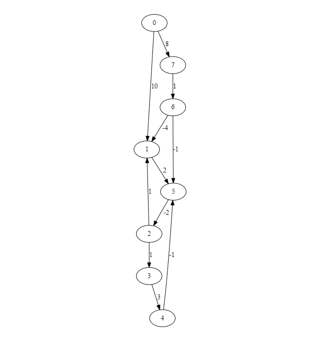
Implementation of Bellman Ford for adjacency matrix

def bellmanford(WMat,s):
    # Initialization
    (rows,cols,x) = WMat.shape
    infinity = np.max(WMat)*rows+1
    distance = {}
    for v in range(rows):
        distance[v] = infinity       
    distance[s] = 0
    
    # Computing shortest distance for each vertex from source
    # Repeat the process n times where n is number of vertices
    for i in range(rows):
        # Check for each adjacent of u vertex
        for u in range(rows):
            for v in range(cols):
                if WMat[u,v,0] == 1:
                        # If distance of v through u is smaller than the current distance of v, then update
                    if distance[u] + WMat[u,v,1] < distance[v]:
                        distance[v] = distance[u] + WMat[u,v,1]
    return(distance)


edges = [(0,1,10),(0,7,8),(1,5,2),(2,1,1),(2,3,1),(3,4,3),(4,5,-1),(5,2,-2),(6,1,-4),(6,5,-1),(7,6,1)]
size = 8
import numpy as np
W = np.zeros(shape=(size,size,2))
for (i,j,w) in edges:
    W[i,j,0] = 1
    W[i,j,1] = w    
print(bellmanford(W,0))

Output

{0: 0, 1: 5.0, 2: 5.0, 3: 6.0, 4: 9.0, 5: 7.0, 6: 9.0, 7: 8.0}

Complexity

$O(V^3 )$ - where $V$ is number of vertices.

 

Implementation of Bellman Ford for adjacency list

def bellmanfordlist(WList,s):
    # Initialization
    infinity = 1 + len(WList.keys())*max([d for u in WList.keys() for (v,d) in WList[u]])
    distance = {}
    for v in WList.keys():
        distance[v] = infinity        
    distance[s] = 0
    
    # Computing shortest distance for each vertex from source
    # Repeat the process n times where n is number of vertices   
    for i in WList.keys():
        # Check for each adjacent of u vertex
        for u in WList.keys():
            for (v,d) in WList[u]:
                # If distance of v through u is smaller than the current distance of v, then update
                if distance[u] + d < distance[v]:
                    distance[v] = distance[u] + d
    return(distance)


edges = [(0,1,10),(0,7,8),(1,5,2),(2,1,1),(2,3,1),(3,4,3),(4,5,-1),(5,2,-2),(6,1,-4),(6,5,-1),(7,6,1)]
size = 8
WL = {}
for i in range(size):
    WL[i] = []
for (i,j,d) in edges:
    WL[i].append((j,d))
print(bellmanfordlist(WL,0))

Output

{0: 0, 1: 5, 2: 5, 3: 6, 4: 9, 5: 7, 6: 9, 7: 8}

 

Code Execution Flow

 

Complexity

$O(V*E )$- where $E$ is number of edges and $V$ is number of vertices.

 

---

 

All pair of shortest path

• Find the shortest paths between every pair of vertices i and j.
• It is equivalent to if run Dijkstra or Bellman-Ford from each vertex.

Floyd-Warshall algorithm

The Floyd-Warshall algorithm is an efficient algorithm for finding the shortest path between all pairs of nodes in a weighted graph. Some important points and properties of the Floyd-Warshall algorithm are:

1. All-pairs shortest path: The Floyd-Warshall algorithm computes the shortest path between all pairs of nodes in the graph.
2. Negative cycles: The Floyd-Warshall algorithm can detect negative cycles in the graph. A negative cycle is a cycle in the graph where the sum of the weights of the edges is negative. If there is a negative cycle in the graph, then the algorithm will report that there is a negative cycle.
3. Dynamic programming: The Floyd-Warshall algorithm uses dynamic programming to compute the shortest path between all pairs of nodes in the graph. The algorithm builds a table of shortest paths between pairs of nodes by iteratively considering intermediate nodes along the path.
4. No guarantee of uniqueness: The shortest path between two nodes in a graph may not be unique. If there are multiple shortest paths between two nodes, then the Floyd-Warshall algorithm may return any one of them.
5. Floyd-Warshall's works for both directed and undirected graphs with non-negative edges weights.
6. Floyd-Warshall's does not work with an undirected graph with negative edges weight, as it will be declared as a negative weight cycle.

 

Algorithm Steps

Here are the steps for the algorithm:

1. Initialization: Create a 2-dimensional array SP of size n x n, where n is the number of vertices in the graph. For each pair of vertices (i,j), initialize SP[i][j] to the weight of the edge from vertex i to vertex j. If there is no edge between vertices i and j, then set SP[i][j] to infinity.

2. For each vertex k from 1 to n, compute the shortest path between every pair of vertices (i,j) that passes through k. To do this, update SP[i][j] as follows:

   SP[i][j] = min(SP[i][j], SP[i][k] + SP[k][j])

   This means that the shortest path from vertex i to vertex j that passes through k is the minimum of the current shortest path from i to j and the sum of the shortest path from i to k and the shortest path from k to j.

3. After the step 2 is complete, the SP array will contain the shortest path between every pair of vertices in the graph.

 

For given input graph

 

Implementation of Floyd Warshall Algorithm

def floydwarshall(WMat):
    # Initialization
    (rows,cols,x) = WMat.shape
    infinity = float('inf')  
    SP = np.zeros(shape=(rows,cols,cols+1))
    
        # Filling the initial graph entry in matrix
    for i in range(rows):
        for j in range(cols):
            if WMat[i,j,0] == 1:
                SP[i,j,0] = WMat[i,j,1]
            else:
                SP[i,j,0] = infinity
    
    # Repeat the process n times where n is number of vertices
    for k in range(1,cols+1):
        # Checking The shortest path distance for each pair in matrix 
        for i in range(rows):
            for j in range(cols):
                SP[i,j,k] = min(SP[i,j,k-1],SP[i,k-1,k-1]+SP[k-1,j,k-1])
    
    # Retuen the last updated matrix
    return(SP[:,:,cols])


edges = [(0,1,10),(0,7,8),(1,5,2),(2,1,1),(2,3,1),(3,4,3),(4,5,-1),(5,2,-2),(6,1,-4),(6,5,-1),(7,6,1)]
size = 8
import numpy as np
W = np.zeros(shape=(size,size,2))
for (i,j,w) in edges:
    W[i,j,0] = 1
    W[i,j,1] = w    
print(floydwarshall(W))

Output

[[inf  5.  5.  6.  9.  7.  9.  8.]
    [inf  1.  0.  1.  4.  2. inf inf]
    [inf  1.  1.  1.  4.  3. inf inf]
    [inf  1.  0.  1.  3.  2. inf inf]
    [inf -2. -3. -2.  1. -1. inf inf]
    [inf -1. -2. -1.  2.  1. inf inf]
    [inf -4. -4. -3.  0. -2. inf inf]
    [inf -3. -3. -2.  1. -1.  1. inf]]

Complexity

$O(V^3 )$ - where $V$ is number of vertices.

 

---

 

Spanning Tree(ST)

• Retain a minimal set of edges so that graph remains connected
• Recall that a minimally connected graph is a tree
• Adding an edge to a tree creates a loop
• Removing an edge disconnects the graph
• Want a tree that connects all the vertices — spanning tree
• More than one spanning tree, in general

Minimum Cost Spanning Tree(MCST)

• Add the cost of all the edges in the tree

• Among the different spanning trees, choose one with minimum cost

• Some facts about trees

  • A tree on n vertices has exactly n − 1 edges
  • Adding an edge to a tree must create a cycle.
  • In a tree, every pair of vertices is connected by a unique path

Algorithms:-

• Prim's Algorithm
• Kruskal's Algorithm

 

Prim's Algorithm

Prim's algorithm is a greedy algorithm that finds a minimum spanning tree (MST) for a weighted undirected graph. Here are some of the key points or properties of Prim's algorithm:

1. Greedy approach: Prim's algorithm is a greedy algorithm that works by building up the MST one vertex at a time, always choosing the cheapest edge that connects the growing tree to an outside vertex.
2. Works on connected graphs: Prim's algorithm only works on connected graphs, meaning that there must be a path between any two vertices in the graph.
3. Weighted edges: Prim's algorithm requires that the graph have weighted edges. The weights represent the cost or distance of traveling between two vertices.
4. Spanning tree: Prim's algorithm always produces a spanning tree, which is a subset of the edges that connects all vertices in the graph and contains no cycles.
5. Unique solution: If the weights of the edges are unique, then the MST produced by Prim's algorithm is unique.

 

Algorithm Steps

Here are the steps for the algorithm:

1. Choose any vertex as the starting vertex and add it to the MST set. Initialize the weight of this vertex to 0.
2. Find the edge with the minimum weight that connects the starting vertex to any other vertex.
3. Add the adjacent vertex connected by the minimum weight edge to the MST set. Set its weight to the weight of the edge.
4. Repeat steps 2 and 3 until all vertices are included in the MST set.

 

Working Visualization

Open Visualization

Select Prim's Algorithm from bottom-left menu

 

Source:- https://visualgo.net/en/mst

 

For given input graph

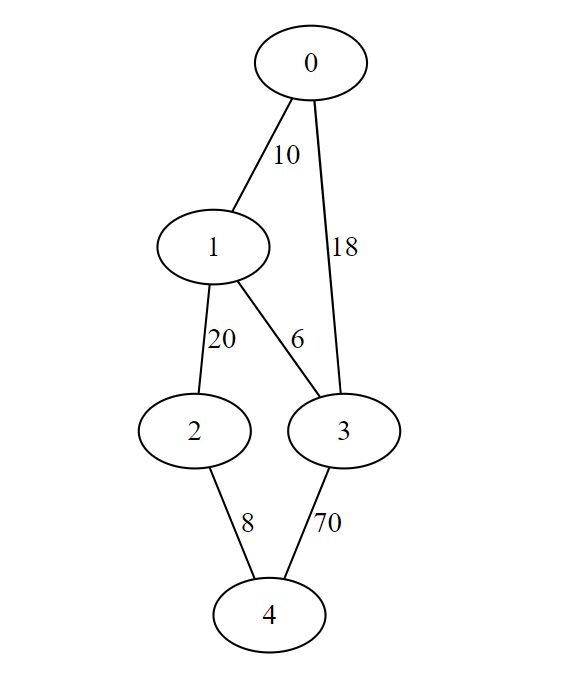
Implementation of Prim's Algorithm

def primlist(WList):
    # Initialization
    infinity = 1 + max([d for u in WList.keys() for (v,d) in WList[u]])
    (visited,distance,TreeEdges) = ({},{},[])
    for v in WList.keys():
        (visited[v],distance[v]) = (False,infinity)
    
    # Start from vertex 0, marked visited and update the distance of adjacents from 0
    visited[0] = True
    for (v,d) in WList[0]:
        distance[v] = d
    
    # Repeat the below process (number of vertices-1) times
    for i in range(1,len(WList.keys())):
        mindist = infinity
        nextv = None
        #Finding the minimum weight edge (u,v) where vertex u is visited and v is not visited 
        for u in WList.keys():
            for (v,d) in WList[u]:
                if visited[u] and (not visited[v]) and d < mindist:
                    mindist = d
                    nextv = v
                    nexte = (u,v)
        
        # Mark nextv as visited and append the nexte in MST
        visited[nextv] = True
        TreeEdges.append(nexte)
        
        # Update the distance of unvisited adjacents of nextv if smaller than current
        for (v,d) in WList[nextv]:
            if not visited[v]:
                if d < distance[v]:
                    distance[v] = d
    return(TreeEdges)


dedges = [(0,1,10),(0,3,18),(1,2,20),(1,3,6),(2,4,8),(3,4,70)]
edges = dedges + [(j,i,w) for (i,j,w) in dedges]
size = 5
WL = {}
for i in range(size):
    WL[i] = []
for (i,j,d) in edges:
    WL[i].append((j,d))
print(primlist(WL))

Output

[(0, 1), (1, 3), (1, 2), (2, 4)]

Output minimum spanning tree with cost 44

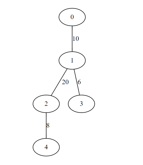
Code Execution Flow

 

 

Other Implementation

def primlist2(WList):
    # Initialization
    infinity = float("inf")
    (visited,distance,nbr) = ({},{},{})
    for v in WList.keys():
        (visited[v],distance[v],nbr[v]) = (False,infinity,-1)
    
    # Set start vertex distance to 0 
    distance[0] = 0
        
    # Repeat the below process (number of vertices-1) times
    for i in range(0,len(WList.keys())):
        # Find minimum distance value on vertices which are not visited
        min_dist = min([distance[v] for v in WList.keys() if not visited[v]])
        
        # Find all vertices that have minimum distance value min_dist and not visited
        nextv_list = [v for v in WList.keys() if (not visited[v]) and distance[v] == min_dist]
        
        # Select the minimum level value vertex from nextv_list ans mark visited
        nextv = min(nextv_list)      
        visited[nextv] = True
        
        # Update the nbr or parent value for v with minimum eadge distance
        for (v,d) in WList[nextv]:
            if not visited[v]:
                if d < distance[v]:
                    nbr[v] = nextv
                    distance[v] = d
    return(nbr)



dedges = [(0,1,10),(0,3,18),(1,2,20),(1,3,6),(2,4,8),(3,4,70)]
edges = dedges + [(j,i,w) for (i,j,w) in dedges]
size = 5
WL = {}
for i in range(size):
    WL[i] = []
for (i,j,d) in edges:
    WL[i].append((j,d))
print(primlist2(WL))

Output

{0: -1, 1: 0, 2: 1, 3: 1, 4: 2}

 

Code Execution Flow

 

Complexity

$O(V^2 )$ - where $V$ is number of vertices.

 

---

 

Kruskal's Algorithm

Kruskal's algorithm is a greedy algorithm used to find the minimum spanning tree (MST) of a connected, undirected graph. The algorithm works by iteratively adding the edges of the graph with the smallest weights that do not create a cycle in the MST. Here are some important points and properties of Kruskal's algorithm:

1. Kruskal's algorithm is a greedy algorithm used to find the minimum spanning tree (MST) of a connected, undirected graph.
2. The algorithm works by iteratively adding the edges of the graph with the smallest weights that do not create a cycle in the MST.
3. Kruskal's algorithm guarantees that the MST is unique if the graph has unique edge weights.

 

Algorithm Steps

Here are the steps for the of Kruskal's algorithm:

1. Sort all the edges of the graph in non-decreasing order of their weights.
2. Create a new empty set for the minimum spanning tree (MST).
3. Iterate through the sorted edges, starting with the edge with the smallest weight.
4. For each edge, check if adding it to the MST will create a cycle.
5. If the edge does not create a cycle, add it to the MST.
6. Repeat steps 4 and 5 until all vertices are included in the MST, or until the desired number of edges have been added.
7. Return the MST.

 

Working Visualization

Open Visualization

Select Kruskal's Algorithm from bottom-left menu

 

Source:- https://visualgo.net/en/mst

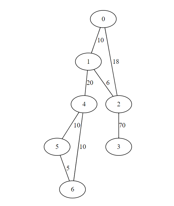
For given input graph

Implementation of Kruskal's Algorithm

def kruskal(WList):
    # Initialization
    (edges,component,TE) = ([],{},[])
    for u in WList.keys():
        # Weight as first value in tuple to sort easily
        edges.extend([(d,u,v) for (v,d) in WList[u]])
        # Initially each vertex as single components and assign leader of each component 
        component[u] = u
    
    # Sort the edges in increasing order of their weights
    edges.sort()
    
    for (d,u,v) in edges:
        # If (u,v) edge is not creating the cycle in MST, add the edge in MST
        if component[u] != component[v]:
            TE.append((u,v))
            c = component[u]
            # Update of component leader 
            for w in WList.keys():
                if component[w] == c:
                    component[w] = component[v]
    return(TE)


dedges = [(0,1,10),(0,2,18),(1,2,6),(1,4,20),(2,3,70),(4,5,10),(4,6,10),(5,6,5)]
edges = dedges + [(j,i,w) for (i,j,w) in dedges]
size = 7
WL = {}
for i in range(size):
    WL[i] = []
for (i,j,d) in edges:
    WL[i].append((j,d))
print(kruskal(WL))

Output

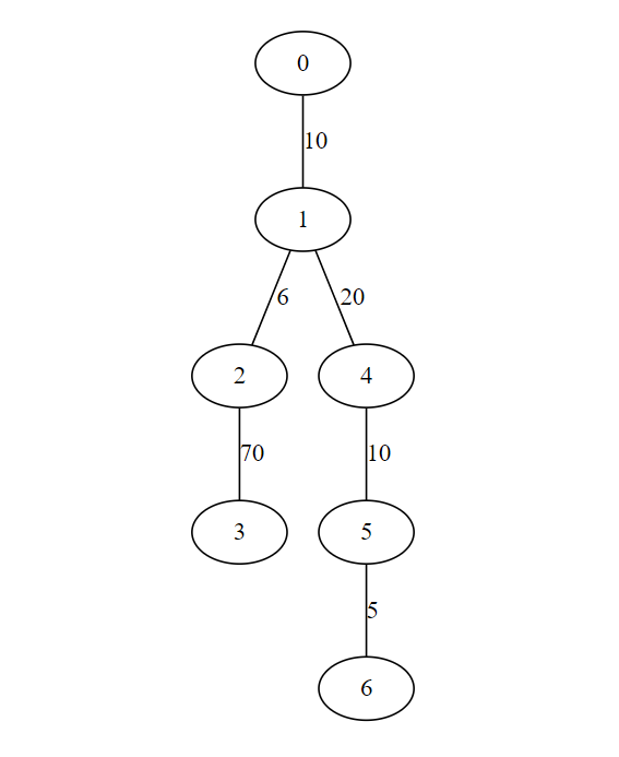
[(5, 6), (1, 2), (0, 1), (4, 5), (1, 4), (2, 3)]

Output minimum spanning tree with cost 121

Code Execution Flow

 

Complexity

$O(V^2 )$ - where $V$ is number of vertices.