---

Home Week-1 Week-3

---

PDSA - Week 2

Complexity

The complexity of an algorithm is a function describing the efficiency of the algorithm in terms of the amount of input data. There are two main complexity measures of the efficiency of an algorithm:

Space complexity

The space complexity of an algorithm is the amount of memory it needs to run to completion.

Generally, space needed by an algorithm is the sum of the following two components:

• Fixed part($C$$C$) - Size of code

• Variable Part($S_x$$S_x$) - Depend on input size, to store in memory

  Total Space $(T(x))=C+S_x$$(T(x)) = C + S_x$

Time complexity

The time complexity of an algorithm is the amount of computer time it needs to run to completion. Computer time represents the number of operations executed by the processor.

Time complexity calculated in three types of cases:

• Best case

• Average case

• Worst Case

Growth rate of functions

The number of operations for an algorithm is usually expressed as a function of the input.

For Example:

1
s = 0 #1
2
For i in range(n): #n+1
3
    for j in range(n): #n(n+1)
4
        s = s + 1 #n^2
5
print(s)#1

Function for given code is :

$f(n)=2n^2+2n+3$$f(n) = 2n^2 + 2n + 3$

Ignore all the constant and coefficient just look at the highest order term in relation to $n$$n$. So $f(n)$$f(n)$ is proportional to $n^2$$n^2$

 

Notations to represent complexity

The notation are mathematical notations that are commonly used to describe the time complexity of an algorithm or the upper and lower bounds of how an algorithm's running time grows as the input size grows.

Big-Oh($O$$O$) - Upper bound:

Big $O$$O$ notation describes the upper bound of an algorithm's running time. Specifically, we use the notation $O(f(n))$$O(f(n))$ to describe the maximum growth rate of an algorithm's running time. This means that the algorithm's running time will not grow faster than some constant multiple of $f(n)$$f(n)$ as the input size grows.

Omega($\mathrm{\Omega }$$\Omega$) - Lower bound:

Omega notation, on the other hand, describes the lower bound of an algorithm's running time. Specifically, we use the notation $\Omega (f(n))$$Ω(f(n))$ to describe the minimum growth rate of an algorithm's running time. This means that the algorithm's running time will not grow slower than some constant multiple of $f(n)$$f(n)$as the input size grows.

Theta($\mathrm{\Theta }$$\Theta$) - Tightly bound:

Theta notation describes both the upper and lower bounds of an algorithm's running time. Specifically, we use the notation $\Theta (f(n))$$Θ(f(n))$ to describe the tight bound of an algorithm's running time. This means that the algorithm's running time will grow at the same rate as some constant multiple of $f(n)$$f(n)$ as the input size grows.

 

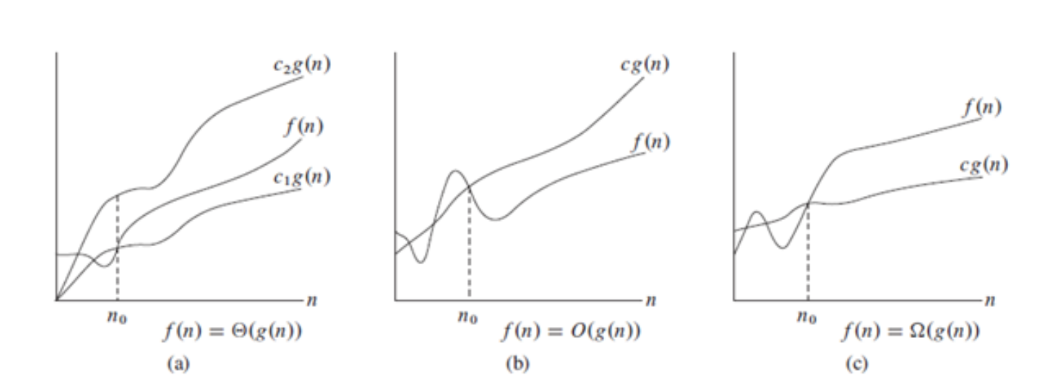
source = https://mitpress.mit.edu/9780262046305/introduction-to-algorithms/

It's important to note that big O notation describes the upper bound of the growth rate of a function. Some algorithms may have a best-case or average-case time complexity that is much faster than their worst-case time complexity. However, the worst-case time complexity is typically what is used to describe the time complexity of an algorithm.

We often use "big O" notation to describe the growth rate of functions. This notation allows us to compare the time complexity of algorithms and the behavior of functions as their input size grows to infinity.

Here are some common functions and their growth rates, listed from slowest-growing to fastest-growing:

• $O(1)$$O(1)$ - constant time

• $O(logn)$$O(log n)$ - logarithmic time

• $O(n)$$O(n)$ - linear time

• $O(nlogn)$$O(n log n)$ - linearithmic time

• $O(n^2)$$O(n^2)$ - quadratic time

• $O(n^3)$$O(n^3)$ - cubic time

• $O(2^n)$$O(2^n)$ - exponential time

• $O(n!)$$O(n!)$ - factorial time

The growth rate of a function is important when analyzing the time complexity of an algorithm. For example, if an algorithm has a time complexity of $O(n^2)$$O(n^2)$, it means that its running time grows quadratically with the input size. If the input size doubles, the running time will increase by a factor of four.

 

Calculate complexity

xxxxxxxxxx
4
1
a = 10
2
b = 20
3
s = a + b
4
print(s)

Complexity ? $O(1)$$O(1)$

Complexity for single loop

xxxxxxxxxx
3
1
s = 0
2
For i in range(n):
3
    s = s + 1

Complexity ? O(n)

Complexity for nested two loop

xxxxxxxxxx
4
1
s = 0
2
For i in range(n):
3
    for j in range(n):
4
        s = s + 1

Complexity ? $O(n^2)$$O(n^2)$

Complexity for nested three loop

xxxxxxxxxx
5
1
s = 0
2
For i in range(n):
3
    for j in range(n):
4
        for k in range(n)
5
            s = s + 1

Complexity ? $O(n^3)$$O(n^3)$

Complexity for combination of all

xxxxxxxxxx
12
1
s = 0
2
For i in range(n):
3
    s = s + 1
4
s = 0
5
For i in range(n):
6
    for j in range(n):
7
        s = s + 1
8
s = 0
9
For i in range(n):
10
    for j in range(n):
11
        for k in range(n)
12
            s = s + 1

Complexity ? $O(n^3)$$O(n^3)$

 

Complexity for recursive solution

xxxxxxxxxx
4
1
def factorial(n)
2
    if (n == 0):
3
        return 1
4
    return n * factorial(n - 1)

Recurrence relation ? $T(n)=T(n-1)+O(1)=1+1+1...ntimes$$T(n) = T(n-1) + O(1) = 1+1+1...n~ times$

Complexity ? $O(n)$$O(n)$

 

Complexity for recursive solution

xxxxxxxxxx
10
1
def merge(A,B):
2
    #statement block for merging two sorted array
3
def mergesort(A):
4
    n = len(A)
5
    if n <= 1:
6
        return(A)
7
    L = mergesort(A[:n//2])
8
    R = mergesort(A[n//2:])
9
    B = merge(L,R)
10
    return(B) 

Recurrence relation - $T(n)=2T(n/2)+O(n)$$T(n) = 2T(n/2)+ O(n)$

Complexity ? $O(nlogn)$$O(nlogn)$

 

 

Searching Algorithm

Linear search and Binary search working visualization

https://www.cs.usfca.edu/~galles/visualization/Search.html

 

Linear Search or Naïve Search

Implementation

xxxxxxxxxx
5
1
def naivesearch(L,v):
2
  for i in range(len(L)):
3
    if v == L[i]:
4
      return i
5
  return(False)

Analysis

Best Case - $O(1)$$O(1)$

Average Case - $O(n)$$O(n)$

Worst Case - $O(n)$$O(n)$

 

Binary Search

Binary search is an efficient search algorithm used to find the position of a target value within a sorted list. The algorithm compares the target value to the middle element of the list. If the target value is equal to the middle element, the search is complete. Otherwise, the algorithm recursively searches either the left or right half of the list, depending on whether the target value is greater or less than the middle element.

Algorithm:

1. Start with a sorted list and a target value.

2. Set the low and high pointers to the first and last indices of the list, respectively.

3. While the low pointer is less than or equal to the high pointer:

   A. Calculate the middle index as the average of the low and high pointers (round down if necessary).

   B. If the target value is equal to the middle element of the list, return the middle index.

   C. If the target value is less than the middle element, set the high pointer to the index before the middle index.

   D. If the target value is greater than the middle element, set the low pointer to the index after the middle index.

4. If the target value is not found in the list, return False (or some other indication that the value is not present).

 

Iterative Implementation

xxxxxxxxxx
12
1
def binarysearch(L, v):  #v = target element
2
    low = 0
3
    high = len(L) - 1
4
    while low <= high: 
5
        mid = (low + high) // 2
6
        if L[mid ] < v:
7
            low = mid  + 1
8
        elif L[mid ] > v:
9
            high = mid  - 1
10
        else:
11
            return mid
12
    return False

 

Code Execution Flow

 

Recursive Implementation without slicing

xxxxxxxxxx
10
1
def binarysearch(L,v,low,high): #v = target element, low = first index, high = last index
2
    if high - low < 0:
3
        return False
4
    mid = (high + low)//2
5
    if v == L[mid]:
6
        return mid
7
    if v < L[mid]:
8
        return(binarysearch(L,v,low,mid-1))
9
    else:
10
        return(binarysearch(L,v,mid+1,high))

 

Code Execution Flow

 

 

Lecture Implementation (Not recommended to achieve $O(logn)$$O(log~n)$ time

*Due to use of slicing, this implementation takes O(n) time

xxxxxxxxxx
10
1
def binarysearch(L,v):
2
    if L == []:
3
        return(False)
4
    mid = len(L)//2
5
    if v == L[mid]:
6
        return mid
7
    if v < L[mid]:
8
        return(binarysearch(L[:mid],v))
9
    else:
10
        return(binarysearch(L[mid+1:],v))

 

Analysis

Best Case - $O(1)$$O(1)$

Average Case - $O(logn)$$O(logn)$

Worst Case - $O(logn)$$O(logn)$

 

Sorting Algorithm

Selection Sort

Selection sort is a simple sorting algorithm that works by repeatedly finding the minimum element from an unsorted part of the list and placing it at the beginning of the sorted part of the list.

Algorithm:

1. Repeat steps 2-5 for the unsorted part of the list until the entire list is sorted.

2. Set the first element as the minimum value in the remaining unsorted part of the list.

3. Iterate through the unsorted part of the list, comparing each element to the current minimum value.

4. If a smaller element is found, update the minimum value.

5. After iterating through the unsorted part of the list, swap the minimum value with the first element of the unsorted part of the list.

 

Visualization

Select the SELECTION SORT(SEL) option on top bar then run the visualization.

Source - https://visualgo.net/en/sorting

 

Implementation

xxxxxxxxxx
11
1
def selectionsort(L):
2
    n = len(L)
3
    if n < 1:
4
        return(L)
5
    for i in range(n):
6
        minpos = i
7
        for j in range(i+1,n):
8
            if L[j] < L[minpos]:
9
                minpos = j
10
        (L[i],L[minpos]) = (L[minpos],L[i])
11
    return(L)

 

Code Execution Flow

 

 

Analysis

Best Case - $n+(n-1)+(n-2)...2+1=n(n+1)/2=O(n^2)$$n + (n-1) + (n-2)...2 + 1 = n(n+1)/2 = O(n^2)$

Average Case - $n+(n-1)+(n-2)...2+1=n(n+1)/2=O(n^2)$$n + (n-1) + (n-2)...2 + 1 = n(n+1)/2 = O(n^2)$

Worst Case - $n+(n-1)+(n-2)...2+1=n(n+1)/2=O(n^2)$$n + (n-1) + (n-2)...2 + 1 = n(n+1)/2 = O(n^2)$

Stable - No

Sort in Place - Yes

 

Insertion Sort

Insertion sort is a simple sorting algorithm that works by repeatedly iterating through the list, comparing adjacent elements and swapping them if they are in the wrong order.

Algorithm:

1. Iterate through the list from the second element to the end (i.e., the element at index 1 to the last element at index n-1).

2. For each element, compare it with the previous element.

3. If the previous element is greater than the current element, swap the two elements.

4. Continue to compare the current element with the previous element until the previous element is not greater than the current element or the current element is at the beginning of the list.

5. Repeat steps 2-4 for all elements in the list.

 

Visualization

Select the INSERTION SORT(INS) option on top bar then run the visualization.

 

Source - https://visualgo.net/en/sorting

Implementation

xxxxxxxxxx
10
1
def insertionsort(L):
2
    n = len(L)
3
    if n < 1:
4
        return(L)
5
    for i in range(n):
6
        j = i
7
        while(j > 0 and L[j] < L[j-1]):
8
            (L[j],L[j-1]) = (L[j-1],L[j])
9
            j = j-1
10
    return(L)

 

Code Execution Flow

 

Analysis

Best Case - $1+1+1...1+1(ntimes)=n=O(n)$$1 + 1 + 1...1 + 1(n times) = n = O(n)$ - If list is already sorted

Average Case - $n+(n-1)+(n-2)...2+1=n(n+1)/2=O(n^2)$$n + (n-1) + (n-2)...2 + 1 = n(n+1)/2 = O(n^2)$

Worst Case - $n+(n-1)+(n-2)...2+1=n(n+1)/2=O(n^2)$$n + (n-1) + (n-2)...2 + 1 = n(n+1)/2 = O(n^2)$

Stable - Yes

Sort in Place - Yes

 

Merge Sort

Merge sort is a popular sorting algorithm that uses the divide-and-conquer technique. It works by recursively dividing an list into two halves, sorting each half separately, and then merging them back together into a single sorted list.

Algorithm:

1. If the list contains only one element or is empty, it is already sorted. Return the list.

2. Divide the list into two halves, using the middle index as the divider.

3. Recursively sort the left half of the list by applying the merge sort algorithm on it.

4. Recursively sort the right half of the list by applying the merge sort algorithm on it.

5. Merge the two sorted halves back together to form a single sorted list. To do this:

   A. Initialize three pointers: one for the left half, one for the right half, and one for the merged list.

   B. Compare the elements pointed to by the left and right pointers. Choose the smaller element, and add it to the merged list.

   C. Move the pointer of the list from which the chosen element was taken to the next element.

   D. Repeat steps B and C until one of the lists is completely processed.

   E. Add any remaining elements from the other list to the merged list.

6. Return the merged list as the final sorted list.

 

Visualization

Select the MERGE SORT(MER) option on top bar then run the visualization.

 

Source - https://visualgo.net/en/sorting

Implementation

​x
1
def merge(A,B): # Merge two sorted list A and B
2
    (m,n) = (len(A),len(B))
3
    (C,i,j) = ([],0,0)
4
    
5
    #Case 1 :- When both lists A and B have elements for comparing
6
    while i < m and j < n:
7
        if A[i] <= B[j]:
8
            C.append(A[i])
9
            i += 1
10
        else:
11
            C.append(B[j])
12
            j += 1
13
    
14
    #Case 2 :- If list B is over, shift all elements of A to C 
15
    while i < m:
16
        C.append(A[i])
17
        i += 1
18
    
19
    #Case 3 :- If list A is over, shift all elements of B to C 
20
    while j < n:
21
        C.append(B[j])
22
        j += 1
23
    
24
    # Return sorted merged list   
25
    return C
26

27

28

29
# Recursively divide the problem into sub-problems to sort the input list L    
30
def mergesort(L): 
31
    n = len(L)
32
    if n <= 1: #If the list contains only one element or is empty return the list.
33
        return(L)
34
    Left_Half = mergesort(L[:n//2]) #Recursively sort the left half of the list
35
    Right_Half = mergesort(L[n//2:]) #Recursively sort the rightt half of the list
36
    Sorted_Merged_List = merge(Left_Half, Right_Half) # Merge two sorted list Left_Half and Right_Half
37
    return(Sorted_Merged_List)

 

Code Execution Flow

 

 

Analysis

Recurrence relation - $T(n)=2T(n/2)+O(n)$$T(n) = 2T(n/2)+ O(n)$

Best Case - $O(nlogn)$$O(nlogn)$

Average Case - $O(nlogn)$$O(nlogn)$

Worst Case - $O(nlogn)$$O(nlogn)$

Stable - Yes

Sort in Place - No

 

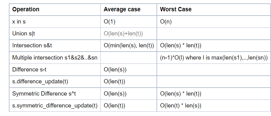
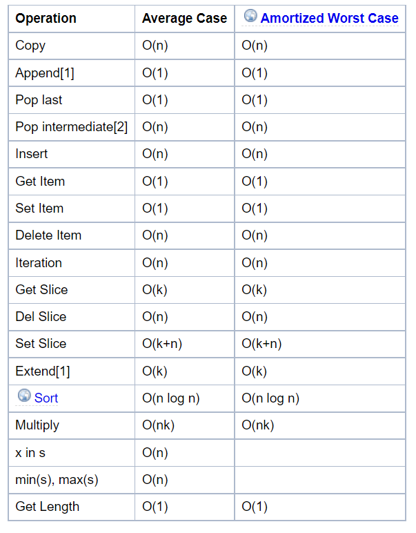
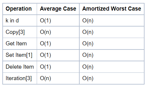
Complexity of python data structure's method

Keep in mind before using for efficiency.

https://wiki.python.org/moin/TimeComplexity

List methods

Dictionary methods

Set Methods