---

Home Week-2 Week-4

---

PDSA - Week 3

Quick Sort

Quick sort is a sorting algorithm that uses the divide-and-conquer strategy to sort the list of elements. The basic idea of quick sort is to partition the input list into two sub-list, one containing elements that are smaller than a chosen pivot element, and the other containing elements that are greater than or equal to the pivot. This process is repeated recursively on each sub-list until the entire list is sorted.

Algorithm:

1. Choose a pivot element from the list. This can be any element, but typically the first or last element is chosen.

2. Partition the list into two sub-list, one containing elements smaller than the pivot, and the other containing elements greater than or equal to the pivot. Steps for Partition:-

   1. Set pivot to the value of the element at the lower index of the list L.

   2. Initialize two indices i and j to lower and lower+1 respectively.

   3. Loop over the range from lower+1 to upper (inclusive) using the variable j.

   4. If the value at index j is less than or equal to the pivot value, increment i and swap the values at indices i and j in the list L.

   5. After the loop, swap the pivot value at index lower with the value at index i in the list L.

   6. Return the index i as the position of the pivot value.

3. Recursively apply steps 1 and 2 to each sub-list until the entire list is sorted.

 

Visualization

Select the Quick Sort(QUI) option on top bar then run the visualization.

Source - https://visualgo.net/en/sorting

 

Implementation

​x
1
def partition(L,lower,upper):
2
  # Select first element as a pivot 
3
  pivot = L[lower]
4
  i = lower
5
  for j in range(lower+1,upper+1):
6
    if L[j] <= pivot:
7
      i += 1
8
      L[i],L[j] = L[j],L[i]
9
  L[lower],L[i]= L[i],L[lower]
10
  # Return the position of pivot
11
  return i
12

13
def quicksort(L,lower,upper):
14
  if(lower < upper):
15
    pivot_pos = partition(L,lower,upper);
16
    # Call the quick sort on leftside part of pivot
17
    quicksort(L,lower,pivot_pos-1)
18
    # Call the quick sort on rightside part of pivot
19
    quicksort(L,pivot_pos+1,upper)
20
  return L

 

Code Execution Flow

 

Lecture Implementation

xxxxxxxxxx
21
1
def quicksort(L,l,r): # Sort L[l:r]
2
    if (r - l <= 1):
3
        return L
4
    (pivot,lower,upper) = (L[l],l+1,l+1)
5
    for i in range(l+1,r):
6
        if L[i] > pivot:
7
            # Extend upper segment
8
            upper = upper+1
9
        else:
10
            # Exchange L[i] with start of upper segment
11
            (L[i], L[lower]) = (L[lower], L[i])
12
            # Shift both segments
13
            (lower,upper) = (lower+1,upper+1)
14
    # Move pivot between lower and upper
15
    (L[l],L[lower-1]) = (L[lower-1],L[l])
16
    lower = lower-1
17
    
18
    # Recursive calls
19
    quicksort(L,l,lower)
20
    quicksort(L,lower+1,upper)
21
    return(L)

 

Code Execution Flow

 

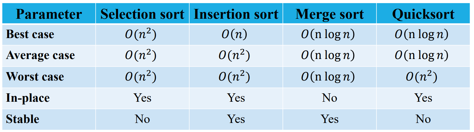
Analysis

Best Case - In each recursive call, If the selected pivot element comes at the middle position and divide the list into two equal halves.

Recurrence relation:- $T(n)=2T(n/2)+O(n)$$T(n) = 2T(n/2)+ O(n)$

Complexity:- $n+n+n...logntimes=nlogn=O(nlogn)$$n + n + n...logn~times = nlogn = O(nlogn)$

 

Worst Case - If the list is already sorted in ascending or descending order (if the selected pivot element comes at the first or last position of the list in each recursive call).

Recurrence relation:- $T(n)=T(n-1)+O(n)$$T(n) = T(n-1)+ O(n)$

Complexity:- $n+(n-1)+(n-2)...1=n(n+1)/2=O(n^2)$$n + (n-1) + (n-2)...1 = n(n+1)/2 = O(n^2)$

 

Average Case

Complexity:- $n+n+n...logntimes=nlogn=O(nlogn)$$n + n + n...logn~times = nlogn = O(nlogn)$

 

Stable - No

Sort in Place - Yes

 

Comparison of sorting algorithm

 

 

Linked List

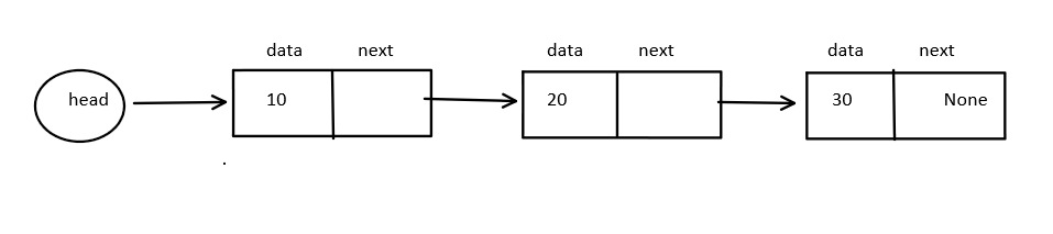
A linked list is a data structure consisting of a sequence of nodes, where each node contains a piece of data and a reference (or pointer) to the next node in the sequence. The first node is called the head, and the last node is called the tail, and the tail node points to null. Linked lists are useful for storing and manipulating collections of data, especially when the size of the collection is not known in advance, as they can dynamically adjust in size.

There are two types of linked lists:

• Singly linked list

• Doubly linked list

Singly linked list

• head:- Store the reference of the first node. If the list is empty, then it stores None

• Each node have two fields:

  • data :- Store actual value

  • next:- Store reference of the next node

 

Representation

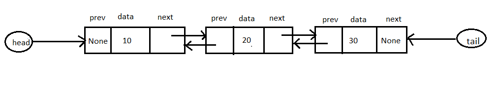
Doubly linked list

• head:- Store the reference of the first node. If the list is empty, then it stores None

• tail:- Store the reference of the last node. If the list is empty, then it stores None

• Each node have three fields:

  • prev:- store reference of the previous node

  • data :- Store actual value

  • next:- Store reference of the next node

 

Representation

 

Visualization of Linked List

Select the Linked List(LL) or Doubly Lined List(DLL) option on top bar then run the visualization.

Source - https://visualgo.net/en/list

 

 

Implementation of singly linked list in Python

Using one class- Recursively

xxxxxxxxxx
77
1
class Node:
2
    def __init__(self, v = None):
3
        self.value = v
4
        self.next = None
5
        return
6
    def isempty(self):
7
        if self.value == None:
8
            return(True)
9
        else:
10
            return(False)
11
    # recursive
12
    def append(self,v):
13
        # If current node is empty
14
        if self.isempty(): 
15
            self.value = v
16
        # If current node is last node of the list 
17
        elif self.next == None:
18
            self.next = Node(v)
19
        # Else raverse to next node
20
        else:
21
            self.next.append(v) 
22
        return
23
    # append, iterative
24
    def appendi(self,v):
25
        # if current node is empty 
26
        if self.isempty():
27
            self.value = v
28
            return
29
        temp = self
30
        # Traverse the list to find the last node
31
        while temp.next != None:
32
            temp = temp.next
33
        temp.next = Node(v) 
34
        return
35
    def insert(self,v):
36
        if self.isempty():
37
            self.value = v
38
            return
39
        newnode = Node(v)
40
        # Exchange values in self and newnode
41
        (self.value, newnode.value) = (newnode.value, self.value)
42
        # Switch links
43
        (self.next, newnode.next) =(newnode, self.next)
44
        return
45
    # delete, recursive
46
    def delete(self,v):
47
        # If list is empty
48
        if self.isempty():
49
            return
50
        # If v is the current node of the list
51
        if self.value == v:
52
            self.value = None
53
            if self.next != None:
54
                self.value = self.next.value
55
                self.next = self.next.next
56
            return
57
        else:
58
            if self.next != None:
59
                self.next.delete(v)
60
                if self.next.value == None:
61
                    self.next = None
62
        return
63
    def display(self):
64
        if self.isempty()==True:
65
            print('None')
66
        else:
67
            temp = self
68
            while temp!=None:
69
                print(temp.value,end="  ")
70
                temp = temp.next
71
head = Node(10)
72
head.append(20)
73
head.append(30)
74
head.appendi(40)
75
head.appendi(50)
76
head.delete(30)
77
head.display()

 

Code Execution Flow

 

 

Using two classes

xxxxxxxxxx
63
1
class Node:
2
    def __init__(self, data):
3
        self.data = data
4
        self.next = None
5

6
class LinkedList:
7
    def __init__(self):
8
        self.head = None
9
    def isempty(self):
10
        if self.head == None: 
11
            return True
12
        else:
13
            return False
14
    def append(self,data):
15
        # If list is empty
16
        if self.isempty():
17
            self.head=Node(data)
18
        else:
19
            temp = self.head
20
            # Traverse the list to find the last node
21
            while temp.next != None:
22
                temp = temp.next
23
            temp.next = Node(data)
24
    def delete(self,v):
25
        # If list is empty
26
        if self.isempty() == True:
27
            return 'List is empty'
28
        # If list have only one element and equal to v
29
        elif self.head.next == None:
30
            # If v is the first node of the list
31
            if self.head.data == v: 
32
                self.head = None
33
            else:
34
                return 'Not exist'
35
        else:
36
            temp = self.head
37
            temp1 = self.head
38
            # Traverse the list to find node with v value
39
            while temp.next!= None and temp.data != v: 
40
                temp1 = temp
41
                temp = temp.next
42
            # If v is the first node of the list
43
            if temp.data == v and temp == self.head: 
44
                self.head = temp.next
45
            # If v is the any node of the list except the first node
46
            elif temp.data == v: 
47
                temp1.next= temp.next
48
            else:
49
                return 'Not exist'
50
    def display(self):
51
        if self.isempty()==True:
52
            print('None')
53
        else:
54
            temp = self.head
55
            while temp!=None:
56
                print(temp.data,end="  ")
57
                temp = temp.next
58
L = LinkedList()
59
L.append(30)
60
L.append(40)
61
L.append(50)
62
L.delete(30)
63
L.display()

 

Code Execution Flow

 

Advantage

• Insertion and deletion operations are easy

• Many complex applications can be easily carried out with linked list concepts like tree, graph, etc.

Disadvantage

• More memory required to store data

• Random access is not possible

Application

• Implementation stack, queue, deque

• Representation of graph.

• Representation of sparse matrix

• Manipulation of the polynomial expression

 

Stack

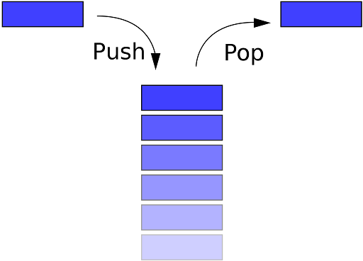
A Stack is a non-primitive linear data structure. It is an ordered list in which the addition of a new data item and deletion of an already existing data item can be done from only one end, known as top of the stack.

The last added element will be the first to be removed from the Stack. That is the reason why stack is also called Last In First Out (LIFO) type of data structure.

 

Basic operations on Stack

Push

The process of adding a new element to the top of the Stack is called the Push operation.

Pop

The process of deleting an existing element from the top of the Stack is called the Pop operation. It returns the deleted value.

Traverse/Display

The process of accessing or reading each element from top to bottom in Stack is called the Traverse operation.

Applications of Stack

• Reverse the string

• Evaluate Expression

• Undo/Redo Operation

• Backtracking

• Depth First Search(DFS) in Graph(Will be discussed in Week-4)

Implementation of the Stack in Python

Stack implementation using a python list

xxxxxxxxxx
22
1
class Stack:
2
    def __init__(self):
3
        self.stack = []
4
    def isempty(self):
5
        return(self.stack == [])
6
    def Push(self,v):
7
        self.stack.append(v)
8
    def Pop(self):
9
        v = None
10
        if not self.isempty():
11
            v = self.stack.pop()
12
        return v    
13
    def __str__(self):
14
        return(str(self.stack))
15
S = Stack()
16
S.Push(10)
17
S.Push(20)
18
S.Push(30)
19
S.Push(40)
20
print(S.Pop())
21
print(S.Pop())
22
print(S)

 

Code Execution Flow

 

Stack implementation using a Linked list

xxxxxxxxxx
50
1
class Node:
2
    def __init__(self, data):
3
        self.data = data
4
        self.next = None
5

6
class Stack:
7
    def __init__(self):
8
        self.top = None
9
        
10
    def isempty(self):
11
        if self.top == None: 
12
            return True
13
        else:
14
            return False
15

16
    def Push(self,data):
17
        if self.isempty():
18
            self.top = Node(data)
19
        else:
20
            temp = Node(data)
21
            temp.next = self.top
22
            self.top = temp
23

24
    def Pop(self):
25
        if self.isempty() == True:
26
            return None
27
        else:
28
            temp = self.top.data
29
            self.top = self.top.next
30
            return temp
31

32
    def display(self):
33
        if self.isempty()==True:
34
            return None
35
        else:
36
            temp = self.top
37
            while temp != None:
38
                print(temp.data)
39
                temp = temp.next        
40

41

42
S = Stack()
43
S.Push(30)
44
S.Push(40)
45
S.Push(50)
46
S.Push(60)
47
S.Push(70)
48
print(S.Pop())
49
print(S.Pop())
50
S.display()

 

Code Execution Flow

 

 

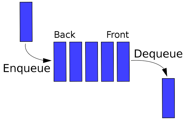
Queue

The Queue is a non-primitive linear data structure. It is an ordered collection of elements in which new elements are added at one end called the Back end, and the existing element is deleted from the other end called the Front end.

A Queue is logically called a First In First Out (FIFO) type of data structure.

 

Basic operations on Queue

Enqueue

The process of adding a new element at the Back end of Queue is called the Enqueue operation.

Dequeue

The process of deleting an existing element from the Front of the Queue is called the Dequeue operation. It returns the deleted value.

Traverse/Display

The process of accessing or reading each element from Front to Back of the Queue is called the Traverse operation.

Applications of Queue

• Spooling in printers

• Job Scheduling in OS

• Waiting list application

• Breadth First Search(BFS) in Graph(Will be discussed in Week-4)

Implementation of the Queue in python

Queue implementation using a python list

xxxxxxxxxx
24
1
class Queue:
2
    def __init__(self):
3
        self.queue = []
4
    def isempty(self):
5
        return(self.queue == []) 
6
    def enqueue(self,v):
7
        self.queue.append(v)   
8
    def dequeue(self):
9
        v = None
10
        if not self.isempty():
11
            v = self.queue[0]
12
            self.queue = self.queue[1:]
13
        return v    
14
    def __str__(self):
15
        return(str(self.queue))
16

17
Q = Queue()
18
Q.enqueue(10)
19
Q.enqueue(20)
20
Q.enqueue(30)
21
Q.enqueue(40)
22
print(Q.dequeue())
23
print(Q.dequeue())
24
print(Q)

 

Code Execution Flow

 

 

Queue implementation using a Linked list

xxxxxxxxxx
60
1
class Node:
2
    def __init__(self, data):
3
        self.data = data
4
        self.next = None
5

6
class Queue:
7
    def __init__(self):
8
        self.front = None
9
        self.rear = None
10
        
11
    def isempty(self):
12
        if self.front == None: 
13
            return True
14
        else:
15
            return False
16

17
    def Enqueue(self,data):
18
        if self.isempty():
19
            self.front = Node(data)
20
            self.rear = self.front
21
        else:
22
            temp = Node(data)
23
            self.rear.next = temp
24
            self.rear = temp
25

26
    def Dequeue(self):
27
        if self.isempty() == True:
28
            return None
29
        elif self.front.next == None:
30
            temp = self.front.data
31
            self.front = None
32
            self.rear = None            
33
        else:
34
            temp = self.front.data
35
            self.front = self.front.next
36
        return temp
37

38
    def display(self):
39
        if self.isempty()==True:
40
            print(None)
41
        else:
42
            temp = self.front
43
            while temp != None:
44
                print(temp.data)
45
                temp = temp.next        
46

47

48
Q = Queue()
49
Q.Enqueue(30)
50
Q.Enqueue(40)
51
Q.Enqueue(50)
52
Q.Enqueue(60)
53
Q.Enqueue(70)
54
print(Q.Dequeue())
55
print(Q.Dequeue())
56
print(Q.Dequeue())
57
print(Q.Dequeue())
58
print(Q.Dequeue())
59
print(Q.Dequeue())
60
Q.display()

 

Code Execution Flow

 

 

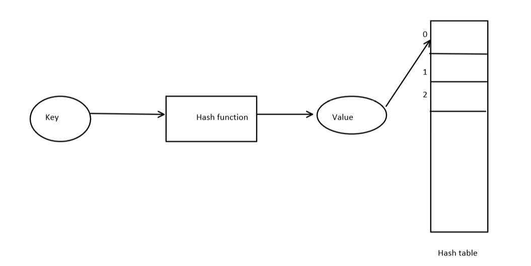
Hash mapping

Hash mapping, also known as hash table or dictionary, is a data structure that allows for efficient insertion, deletion, and retrieval of key-value pairs.

The basic idea behind hash mapping is to use a hash function to map the key to a bucket in an array. The hash function takes the key as input and returns an index of the array where the value corresponding to the key can be stored. When we want to retrieve a value, we simply use the hash function to calculate the index and then access the value stored at that index.

One of the advantages of hash mapping is its constant-time complexity for basic operations such as insertion, deletion, and retrieval, on average, making it efficient for large datasets. However, the performance can be affected by factors such as the quality of the hash function, the number of collisions (i.e., when multiple keys map to the same index), and the size of the array.

 

For storing element

For searching element

Collision

The situation where a newly inserted key maps to an already occupied slot in the hash table is called collision.

Collision resolving technique

Open addressing(Close hashing)

• Linear probing is an open addressing scheme in computer programming for resolving hash collisions in hash tables. Linear probing operates by taking the original hash index and adding successive values linearly until a free slot is found.

  An example sequence of linear probing is:

  h(k)+0, h(k)+1, h(k)+2, h(k)+3 .... h(k)+m-1

  where m is a size of hash table, and h(k) is the hash function.

  Hash function

  Let h(k) = k mod m be a hash function that maps an element k to an integer in [0, m−1], where m is the size of the table. Let the i^th probe position for a value k be given by the function

  h'(k,i) = (h(k) + i) mod m

  The value of i = 0, 1, . . ., m – 1. So we start from i = 0, and increase this until we get a free block in hash table.

   

• Quadratic probing is an open addressing scheme in computer programming for resolving hash collisions in hash tables. Quadratic probing operates by taking the original hash index and adding successive values of an arbitrary quadratic polynomial until an open or empty slot is found.

  An example of a sequence using quadratic probing is:

  $h,h+1,h+4,h+9...h+i^2$$h, h+1, h+4, h+9...h+i^2$

  Quadratic function

  Let h(k) = k mod m be a hash function that maps an element k to an integer in [0, m−1], where m is the size of the table. Let the $i^{th}$$i^{th}$ probe position for a value k be given by the function

  $h(k,i)=(h(k)+c_{1}i+c_2{i}^2)modm$$h(k,i)= (h(k)+c_1i+c_2i^2)~mod~m$

  where c1 and c2 are positive integers. The value of i = 0, 1, . . ., m – 1. So we start from i = 0, and increase this until we get one free slot in hash table.

   

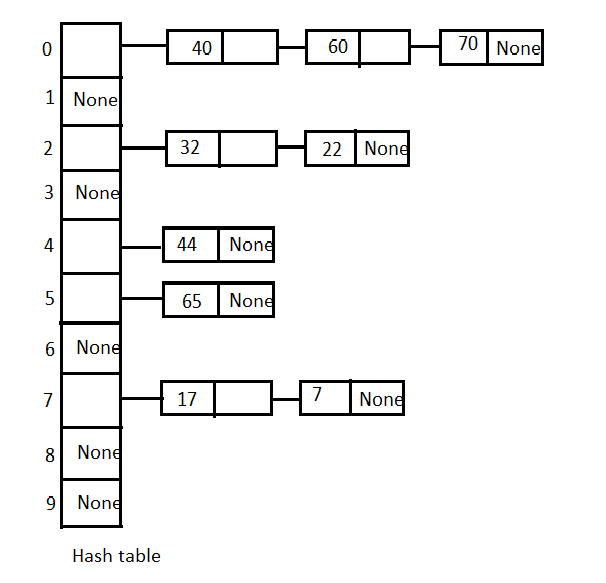
Closed addressing ( Open hashing)

• Separate chaining using linked list: Maintain the separate linked list for each possible generated index by the hash function.

  For example, if the hash function is k mod 10 where k is the key and 10 is the size of the hash table.

 

 

Visualization of Hashing

Source - https://visualgo.net/en/hashtable