Home Week-3 Week-5

PDSA - Week 4

PDSA - Week 4Introduction of GraphBasic Terminology of GraphGraph Representation in data structureFor unweighted directed graphFor unweighted undirected graphGraph Traversing AlgorithmBreadth First Search(BFS) AlgorithmWorking Visualization Implementation BFS for adjacency list of graphImplementation BFS for adjacency matrix of graphDepth First Search(DFS)AlgorithmWorking Visualization Implementation of DFS for adjacency list of graphImplementation of DFS for adjacency matrix of graphApplication of BFS and DFSFind Connected Components in graph using BFSAlgorithmImplementation of Find Connected Components in graph using BFSPre and Post numbering using DFSAlgorithmImplementation of Pre and Post numbering on graph using DFSDirected Acyclic Graph(DAG)Topological SortAlgorithmWorking VisualizationImplementation of Topological Sort for Adjacency listImplementation of Topological Sort for Adjacency matrixLongest Path in DAGAlgorithmWorking VisualizationImplementation for Longest Path on DAGVisualization of graph algorithms using visualgo

Introduction of Graph

Graph:- It is a non-linear data structure. A graph G consist of a non empty set V where members are called the vertices of graph and the set E where member are called the edges.

G = (V, E)

V = set of vertices

E = set of edges

Example:-

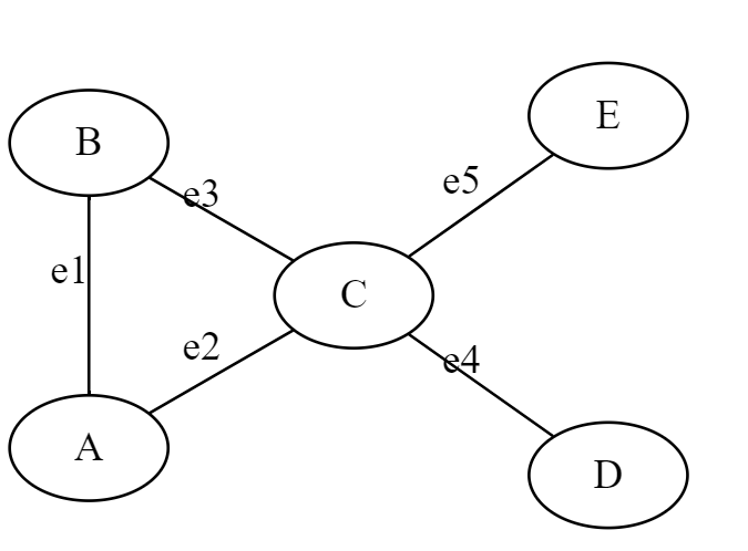
G = (V, E)

V = {A,B,C,D,E}

E = {e1,e2,e3,e4,e5} or {(A,B), (A,C), (B,C), (C,D), (C,E)}

Basic Terminology of Graph

Vertex (or node):

A vertex or node is a fundamental unit in a graph. In a simple graph, each vertex can be connected to other vertices by edges. Vertices are often represented by circles or dots in visual representations of graphs.

Edge:

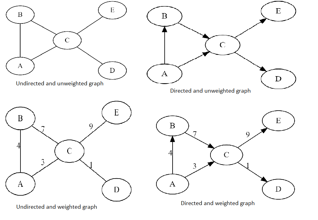
An edge is a line or connection between two vertices in a graph. Edges can be directed or undirected, and weighted or unweighted. In an undirected graph, edges connect vertices without a specified direction, while in a directed graph, edges have a direction, represented by an arrow. In a weighted graph, edges have a numerical weight or value assigned to them.

Degree:

The degree of a vertex is the number of edges that are connected to it. In a directed graph, the degree of a vertex is defined as the sum of the in-degree (number of edges coming into the vertex) and out-degree (number of edges going out of the vertex).

Path:

A path is a sequence of vertices connected by edges. A simple path is a path where no vertex is repeated.

Cycle:

A cycle is a path that starts and ends at the same vertex.

Connectedness:

A graph is said to be connected if there is a path between any two vertices in the graph. A disconnected graph is a graph that is not connected, meaning it can be broken into two or more separate components.

Component:

A component is a connected subgraph of a larger graph. In other words, it is a part of the graph that is connected to other vertices or edges within that part, but not connected to the rest of the graph.

Directed graph:

A directed graph is a graph where edges have a direction, represented by an arrow. In a directed graph, edges are often called arcs.

Undirected graph:

An undirected graph is a graph where edges do not have a direction.

Weighted graph:

A weighted graph is a graph where edges have weights or values assigned to them.

Adjacent vertices:

Two vertices are adjacent if they are connected by an edge.

Incidence:

A vertex is incident on an edge if the vertex is one of the endpoints of the edge.

Subgraph:

A subgraph is a graph that is a subset of another graph, with some edges and vertices removed.

Complete graph:

A complete graph is a graph where every vertex is connected to every other vertex. In other words, there is an edge between every pair of vertices in the graph.

Logical Representation of graph

Graph Representation in data structure

Adjacency matrix:

An adjacency matrix is a two-dimensional array or list that represents a graph. The matrix has a row and column for each vertex, and the value at position (i, j) indicates whether there is an edge between vertices i and j. If there is an edge, the value is 1, and if there is no edge, the value is 0. This representation is useful for dense graphs, where the number of edges is close to the maximum possible number of edges. In python we can use NumPy array or python list for adjacency matrix.

Adjacency list:

An adjacency list is a list of lists where each vertex has a list of its adjacent vertices. Each list contains the vertices that are adjacent to the vertex at that index. This representation is useful for sparse graphs, where the number of edges is much smaller than the maximum possible number of edges. In python we can use dictionary for adjacency list.

For unweighted directed graph

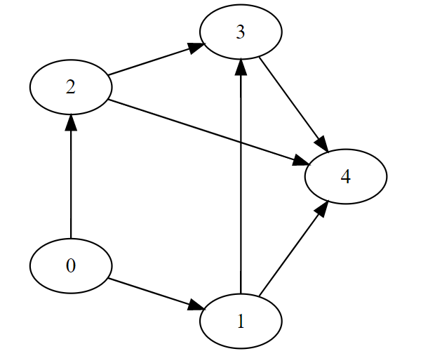
G = (V, E)

V = [0,1,2,3,4]

E = [(0, 1), (0, 2), (1, 3), (1, 4), (2, 4), (2, 3), (3, 4)]

Adjacency matrix representation:

Using NumPy 2d array


1
V = [0,1,2,3,4]
2
E = [(0, 1), (0, 2), (1, 3), (1, 4), (2, 4), (2, 3), (3, 4)] # each tuple(u,v) represent edge from u to v
3
size = len(V)
4
import numpy as np
5
AMat = np.zeros(shape=(size,size))
6
for (i,j) in E:
7
    AMat[i,j] = 1 # mark 1 if edge present in graph from i to j , otherwise 0
8
print(AMat)

Output adjacency matrix (AMat)


xxxxxxxxxx
6
1
[[0. 1. 1. 0. 0.]
2
 [0. 0. 0. 1. 1.]
3
 [0. 0. 0. 1. 1.]
4
 [0. 0. 0. 0. 1.]
5
 [0. 0. 0. 0. 0.]]
6
# AMat[i,j] == 1 represent edge from i to j

Using Python nested list


xxxxxxxxxx
12
1
V = [0,1,2,3,4]
2
E = [(0, 1), (0, 2), (1, 3), (1, 4), (2, 4), (2, 3), (3, 4)]
3
size = len(V)
4
AMat = []
5
for i in range(size):
6
    row = []
7
    for j in range(size):
8
        row.append(0)
9
    AMat.append(row.copy())       
10
for (i,j) in E:
11
    AMat[i][j] = 1 # mark 1 if edge present in graph from i to j , otherwise 0
12
print(AMat)

Output adjacency matrix (AMat)


xxxxxxxxxx
6
1
[[0, 1, 1, 0, 0],
2
[0, 0, 0, 1, 1],
3
[0, 0, 0, 1, 1],
4
[0, 0, 0, 0, 1],
5
[0, 0, 0, 0, 0]]
6
# AMat[i][j] == 1 represent edge from i to j

Adjacency list representation:

Using python dictionary


xxxxxxxxxx
10
1
V = [0,1,2,3,4]
2
E = [(0, 1), (0, 2), (1, 3), (1, 4), (2, 4), (2, 3), (3, 4)]
3
size = len(V)
4
AList = {}
5
# In dictionay AList, for example, AList[i] = [j,k] represent two edge from i to j and i to k
6
for i in range(size):
7
    AList[i] = []
8
for (i,j) in E:
9
    AList[i].append(j)
10
print(AList)

Output adjacency list (AList)


xxxxxxxxxx
2
1
{0: [1, 2], 1: [3, 4], 2: [4, 3], 3: [4], 4: []}
2
# for example, AList[i] = [j,k] represent two edge from i to j and i to k

For unweighted undirected graph

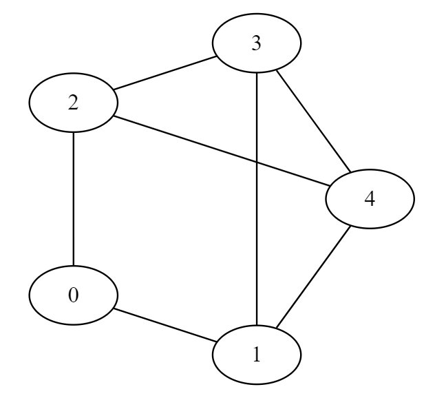
G = (V, E)

V = [0,1,2,3,4]

E = [(0, 1), (0, 2), (1, 3), (1, 4), (2, 4), (2, 3), (3, 4)]

Adjacency matrix representation:

Using NumPy 2d array


xxxxxxxxxx
9
1
V = [0,1,2,3,4]
2
E = [(0, 1), (0, 2), (1, 3), (1, 4), (2, 4), (2, 3), (3, 4)]
3
UE = E + [ (j,i) for (i,j) in E] # each edge represented by two tuple (u,v) and (v,u)
4
size = len(V)
5
import numpy as np
6
AMat = np.zeros(shape=(size,size))
7
for (i,j) in UE:
8
    AMat[i,j] = 1 # mark 1 if edge present in graph from i to j , otherwise 0
9
print(AMat)

Output adjacency matrix (AMat)


xxxxxxxxxx
6
1
[[0. 1. 1. 0. 0.]
2
 [1. 0. 0. 1. 1.]
3
 [1. 0. 0. 1. 1.]
4
 [0. 1. 1. 0. 1.]
5
 [0. 1. 1. 1. 0.]]
6
 # AMat[i,j] == 1 represent edge from i to j

Using Python nested list


xxxxxxxxxx
13
1
V = [0,1,2,3,4]
2
E = [(0, 1), (0, 2), (1, 3), (1, 4), (2, 4), (2, 3), (3, 4)]
3
UE = E + [ (j,i) for (i,j) in E] # each edge represented by two tuple (u,v) and (v,u)
4
size = len(V)
5
AMat = []
6
for i in range(size):
7
    row = []
8
    for j in range(size):
9
        row.append(0)
10
    AMat.append(row.copy())       
11
for (i,j) in UE:
12
    AMat[i][j] = 1 # mark 1 if edge present in graph from i to j , otherwise 0
13
print(AMat)

Output adjacency matrix (AMat)


xxxxxxxxxx
6
1
[[0, 1, 1, 0, 0], 
2
[1, 0, 0, 1, 1], 
3
[1, 0, 0, 1, 1], 
4
[0, 1, 1, 0, 1], 
5
[0, 1, 1, 1, 0]]
6
# AMat[i][j] == 1 represent edge from i to j

Adjacency list representation:

Using python dictionary


xxxxxxxxxx
11
1
V = [0,1,2,3,4]
2
E = [(0, 1), (0, 2), (1, 3), (1, 4), (2, 4), (2, 3), (3, 4)]
3
UE = E + [ (j,i) for (i,j) in E] # each edge represented by two tuple (u,v) and (v,u)
4
size = len(V)
5
AList = {}
6
# In dictionay AList, for example, AList[i] = [j,k] represent two edge from i to j and i to k
7
for i in range(size):
8
    AList[i] = []
9
for (i,j) in UE:
10
    AList[i].append(j)
11
print(AList)

Output adjacency list (AList)


xxxxxxxxxx
2
1
{0: [1, 2], 1: [3, 4, 0], 2: [4, 3, 0], 3: [4, 1, 2], 4: [1, 2, 3]}
2
# for example, AList[i] = [j,k] represent two edge from i to j and i to k

Graph Traversing Algorithm

Graph traversal is the process of visiting all the vertices (nodes) of a graph. There are two commonly used algorithms for graph traversal:

Breadth-First Search (BFS)
Depth-First Search (DFS)

Breadth First Search(BFS)

The Breadth First Search (BFS) algorithm is used to traverse a graph or a tree in a breadth-first manner. BFS starts at the root node and explores all the neighboring nodes at the current depth before moving on to the nodes at the next depth. This is done by using a queue data structure. The algorithm marks each visited node to avoid revisiting it.

Algorithm

Here are the steps for the BFS algorithm:

Choose a starting node and enqueue it to a queue.
Mark the starting node as visited.
While the queue is not empty, dequeue a node from the front of the queue.
For each of the dequeued node's neighbors that are not visited, mark them as visited and enqueue them to the queue.
Repeat steps 3-4 until the queue is empty.

To keep track of the traversal order, you can add each visited node to a list as it is dequeued from the queue.

$O(V^2 )$ $O(V + E)$ $V$ $E$ is number of edges in Graph.

Working Visualization

Implementation BFS for adjacency list of graph


x
1
# Queue Implementation
2
class Queue:
3
    def __init__(self):
4
        self.queue = []
5
    def enqueue(self,v):
6
        self.queue.append(v)
7
    def isempty(self):
8
        return(self.queue == [])    
9
    def dequeue(self):
10
        v = None
11
        if not self.isempty():
12
            v = self.queue[0]
13
            self.queue = self.queue[1:]
14
        return(v)    
15
    def __str__(self):
16
        return(str(self.queue))
17

18
# BFS Implementation For Adjacency list
19
def BFSList(AList,start_vertex):
20
    # Initialization
21
    visited = {}
22
    for each_vertex in AList.keys():
23
        visited[each_vertex] = False    
24
    
25
    # Create Queue object q
26
    q = Queue()
27
    
28
    # Mark the start_vertex visited and insert it into the queue 
29
    visited[start_vertex] = True
30
    q.enqueue(start_vertex)
31
    
32
    # Repeat the following until the queue is empty 
33
    while(not q.isempty()):
34
        # Remove the one vertex from queue
35
        curr_vertex = q.dequeue()
36
        # Visit each adjacent of the removed vertex (if not visited), mark that visited, and insert it into the queue 
37
        for adj_vertex in AList[curr_vertex]:
38
            if (not visited[adj_vertex]):
39
                visited[adj_vertex] = True
40
                q.enqueue(adj_vertex)               
41
    return(visited)
42

43
AList = {0: [1, 2], 1: [3, 4], 2: [4, 3], 3: [4], 4: []}
44
print(BFSList(AList,0))

Output


xxxxxxxxxx
1
1
{0: True, 1: True, 2: True, 3: True, 4: True}

Code Execution Flow

Implementation BFS for adjacency matrix of graph


xxxxxxxxxx
62
1
# Queue Implementation
2
class Queue:
3
    def __init__(self):
4
        self.queue = []
5
    def enqueue(self,v):
6
        self.queue.append(v)
7
    def isempty(self):
8
        return(self.queue == [])
9
    def dequeue(self):
10
        v = None
11
        if not self.isempty():
12
            v = self.queue[0]
13
            self.queue = self.queue[1:]
14
        return(v)    
15
    def __str__(self):
16
        return(str(self.queue))
17

18
# Function to return list of neighbours or adjacent vertex of vertex i
19
def neighbours(AMat,i):
20
    nbrs = []
21
    (rows,cols) = AMat.shape
22
    for j in range(cols):
23
        if AMat[i,j] == 1:
24
            nbrs.append(j)
25
    return(nbrs)
26

27
# BFS Implementation For Adjacency matrix
28
def BFS(AMat,start_vertex):
29
    # Initialization
30
    (rows,cols) = AMat.shape
31
    visited = {}
32
    for each_vertex in range(rows):
33
        visited[each_vertex] = False    
34
    
35
    # Create Queue object q
36
    q = Queue()
37
    
38
    # Mark the start_vertex visited and insert it into the queue 
39
    visited[start_vertex] = True
40
    q.enqueue(start_vertex)
41
    
42
    # Repeat the following until the queue is empty 
43
    while(not q.isempty()):
44
        # Remove the one vertex from queue
45
        curr_vertex = q.dequeue()
46
        # Visit the each adjacent of removed vertex(if not visited) and insert into the queue
47
        for adj_vertex in neighbours(AMat,curr_vertex):
48
            if (not visited[adj_vertex]):
49
                visited[adj_vertex] = True
50
                q.enqueue(adj_vertex)
51
                
52
    return(visited)
53

54

55
V = [0,1,2,3,4]
56
E = [(0, 1), (0, 2), (1, 3), (1, 4), (2, 4), (2, 3), (3, 4)] 
57
size = len(V)
58
import numpy as np
59
AMat = np.zeros(shape=(size,size))
60
for (i,j) in E:
61
    AMat[i,j] = 1
62
print(BFS(AMat,0))

Output


xxxxxxxxxx
1
1
{0: True, 1: True, 2: True, 3: True, 4: True}

Code Execution Flow

Find parent of each vertex using BFS

Parent information is useful to determine shortest path from vertex v in term of number of edges or vertex in path.


xxxxxxxxxx
50
1
# Queue Implementation
2
class Queue:
3
    def __init__(self):
4
        self.queue = []
5
    def enqueue(self,v):
6
        self.queue.append(v)
7
    def isempty(self):
8
        return(self.queue == [])
9
    def dequeue(self):
10
        v = None
11
        if not self.isempty():
12
            v = self.queue[0]
13
            self.queue = self.queue[1:]
14
        return(v)    
15
    def __str__(self):
16
        return(str(self.queue))
17

18
# Using BFS approch For Adjacency list, for path, maintaining the parent of each vertex
19
# Path can be found by backtracking from destination to source using parent information
20
def BFSListPath(AList,start_vertex):
21
    # Initialization
22
    (visited,parent) = ({},{})
23
    for each_vertex in AList.keys():
24
        visited[each_vertex] = False
25
        parent[each_vertex] = -1   
26
    
27
    # Create Queue object q
28
    q = Queue()
29
    
30
    # Mark the start_vertex visited and insert it into the queue 
31
    visited[start_vertex] = True
32
    q.enqueue(start_vertex)
33
    
34
    # Repeat the following until the queue is empty
35
    while(not q.isempty()):
36
        # Remove the one vertex from queue
37
        curr_vertex = q.dequeue()
38
        # Visit the each adjacent of removed vertex(if not visited) and insert into the queue
39
        for adj_vertex in AList[curr_vertex]:
40
            if (not visited[adj_vertex]):
41
                visited[adj_vertex] = True
42
                # Assigne the curr_vertex as parent of each unvisited adjacent of curr_vertex
43
                parent[adj_vertex] = curr_vertex
44
                q.enqueue(adj_vertex)
45
                
46
    return(visited,parent)
47

48

49
AList ={0: [1, 2], 1: [3, 4], 2: [4, 3], 3: [4], 4: []}
50
print(BFSListPath(AList,0))

Output


xxxxxxxxxx
1
1
({0: True, 1: True, 2: True, 3: True, 4: True}, {0: -1, 1: 0, 2: 0, 3: 1, 4: 1})

Find level number of vertices using BFS

Maintain level information to record length of the shortest path, in terms of number of edges or vertex.


xxxxxxxxxx
51
1
# Queue Implementation
2
class Queue:
3
    def __init__(self):
4
        self.queue = []
5
    def enqueue(self,v):
6
        self.queue.append(v)
7
    def isempty(self):
8
        return(self.queue == [])
9
    def dequeue(self):
10
        v = None
11
        if not self.isempty():
12
            v = self.queue[0]
13
            self.queue = self.queue[1:]
14
        return(v)    
15
    def __str__(self):
16
        return(str(self.queue))
17

18
# Using BFS approch For Adjacency list, for path, maintaining the parent of each vertex
19
# Using BFS approch maintaing the adjacent level number from source vertrex
20
def BFSListPathLevel(AList,v):
21
    # Initialization
22
    (level,parent) = ({},{})
23
    for each_vertex in AList.keys():
24
        level[each_vertex] = -1
25
        parent[each_vertex] = -1
26
    
27
    # Create Queue object q
28
    q = Queue()
29
    
30
    # Assigning the level 0 for start_vertex and insert it into the queue
31
    level[v] = 0
32
    q.enqueue(v)
33
    
34
    # Repeat the following until the queue is empty
35
    while(not q.isempty()):
36
        # Remove the one vertex from queue
37
        curr_vertex = q.dequeue()
38
        # Visit the each adjacent of curr_vertex(if level value is -1) and insert into the queue
39
        for adj_vertex in AList[curr_vertex]:
40
            if (level[adj_vertex] == -1):
41
                # Assign the level value on each adjacent one more than the curr_vertex level
42
                level[adj_vertex] = level[curr_vertex] + 1
43
                # Assigne the curr_vertex as parent of adjacent vertex of curr_vertex
44
                parent[adj_vertex] = curr_vertex
45
                q.enqueue(adj_vertex)
46
                
47
    return(level,parent)
48

49

50
AList ={0: [1, 2], 1: [3, 4], 2: [4, 3], 3: [4], 4: []}
51
print(BFSListPathLevel(AList,0))

Output


xxxxxxxxxx
1
1
({0: 0, 1: 1, 2: 1, 3: 2, 4: 2}, {0: -1, 1: 0, 2: 0, 3: 1, 4: 1})

Depth First Search(DFS)

The Depth First Search (DFS) algorithm is used to traverse a graph or a tree in a depth-first manner, exploring as far as possible along each branch before backtracking. This is done by using a stack data structure.

Algorithm

Here are the steps for the Recursive DFS algorithm:

Choose a starting node and mark it as visited.
For each unvisited neighbor of the starting node, recursively call the DFS algorithm starting from that neighbor.
Repeat step 2 for all unvisited neighbors.

Here are the steps for DFS using a stack:

Create a stack S and a set visited to keep track of visited nodes.
Push the starting node onto the stack S.
While S is not empty, pop the top element u from S.
If u is not visited, mark it as visited and do the following:
- Perform any processing on the node u.
- Get all unvisited neighbors v of u and push them onto S.
Repeat steps 3-4 until S is empty.

To keep track of the traversal order, you can add each visited node to a list as it is visited.

$O(V^2 )$ $O(V + E)$ $V$ $E$ is number of edges in Graph.

Working Visualization

Implementation of DFS for adjacency list of graph

DFS using Stack for adjacency list of graph


xxxxxxxxxx
45
1
# Stack Implementation
2
class Stack:
3
    def __init__(self):
4
        self.stack = []
5
    def Push(self,v):
6
        self.stack.append(v)
7
    def isempty(self):
8
        return(self.stack == [])
9
    def Pop(self):
10
        v = None
11
        if not self.isempty():
12
            v = self.stack.pop()
13
        return(v)    
14
    def __str__(self):
15
        return(str(self.stack))
16

17
# DFS Implementation for Adjacency list
18
def DFSList(AList,start_vertex):
19
    # Initializaion
20
    visited = {}
21
    for each_vertex in AList.keys():
22
        visited[each_vertex] = False    
23
    
24
    # Create stack object st
25
    st = Stack()
26
    
27
    # Push start_vertex in to the stack as first vertex
28
    st.Push(start_vertex)    
29
    
30
    # Repeat the following until the stack is empty
31
    while(not st.isempty()):
32
        # Pop one vertex from stack 
33
        current_vertex = st.Pop()
34
        # If popped vertex is not visited, marked visited
35
        if visited[current_vertex] == False:
36
            visited[current_vertex] = True
37
            # Push all unvisited adjacent of popped vertex into the stack
38
            for adj_veretx in AList[current_vertex]:
39
                 if(not visited[adj_veretx]):
40
                     st.Push(adj_veretx)    
41
    return(visited)
42

43

44
AList ={0: [1, 2], 1: [3, 4], 2: [4, 3], 3: [4], 4: []}
45
print(DFSList(AList,0))

Output


xxxxxxxxxx
1
1
{0: True, 1: True, 2: True, 3: True, 4: True}

Code Execution Flow

DFS Recursive (without using external stack)


xxxxxxxxxx
27
1
# Initialization Function
2
def DFSInitList(AList):
3
    (visited,parent) = ({},{})
4
    for each_vertex in AList.keys():
5
        visited[each_vertex] = False
6
        parent[each_vertex] = -1
7
    return(visited,parent)
8

9
# DFS Recursive Implementation for Adjacency list
10
def DFSList(AList,visited,parent,v):
11
    # Mark vertex v as visited vertex
12
    visited[v] = True
13
    # Repeat following for each unvisited adjacent of vertex v
14
    for adj_vertex in AList[v]:
15
        if (not visited[adj_vertex]):
16
            # Assign vertex v as parent of each unvisited adjacent of v 
17
            parent[adj_vertex] = v
18
            
19
            # Recursively call the DFS on unvisited adjacent of v
20
            (visited,parent) = DFSList(AList,visited,parent,adj_vertex)
21
            
22
    return(visited,parent)
23

24

25
AList ={0: [1, 2], 1: [3, 4], 2: [4, 3], 3: [4], 4: []}
26
v,p = DFSInitList(AList)
27
print(DFSList(AList,v,p,0))

Output


xxxxxxxxxx
1
1
({0: True, 1: True, 2: True, 3: True, 4: True}, {0: -1, 1: 0, 2: 0, 3: 1, 4: 3})

Code Execution Flow

DFS global for adjacency list of graph


xxxxxxxxxx
28
1
# Global variable
2
(visited,parent) = ({},{})
3

4
# Initialization function
5
def DFSInitListGlobal(AList):   
6
    for each_vertex in AList.keys():
7
        visited[each_vertex] = False
8
        parent[each_vertex] = -1
9
    return
10

11
# DFS Recursive Implementation for Adjacency list
12
def DFSListGlobal(AList,v):
13
    # Mark vertex v as visited vertex
14
    visited[v] = True
15
    # Repeat following for each unvisited adjacent of vertex v
16
    for adj_vertex in AList[v]:
17
        if (not visited[adj_vertex]):
18
            # Assign vertex v as parent of each unvisited adjacent of v 
19
            parent[adj_vertex] = v
20
            # Recursively call the DFS on unvisited adjacent of v
21
            DFSListGlobal(AList,adj_vertex)                
22
    return
23

24

25
AList ={0: [1, 2], 1: [3, 4], 2: [4, 3], 3: [4], 4: []}
26
DFSInitListGlobal(AList)
27
DFSListGlobal(AList,0)
28
print(visited,parent)

Output


xxxxxxxxxx
1
1
{0: True, 1: True, 2: True, 3: True, 4: True} {0: -1, 1: 0, 2: 0, 3: 1, 4: 3}

Implementation of DFS for adjacency matrix of graph


xxxxxxxxxx
42
1
# Function to return list of neighbours or adjacent vertex of vertex i
2
def neighbours(AMat,i):
3
    nbrs = []
4
    (rows,cols) = AMat.shape
5
    for j in range(cols):
6
        if AMat[i,j] == 1:
7
            nbrs.append(j)
8
    return(nbrs)
9

10
# Initialization Function
11
def DFSInit(AMat):
12
    (rows,cols) = AMat.shape
13
    (visited,parent) = ({},{})
14
    for each_vertex in range(rows):
15
        visited[each_vertex] = False
16
        parent[each_vertex] = -1
17
    return(visited,parent)
18

19
# DFS Recursive Implementation for Adjacency matrix
20
def DFS(AMat,visited,parent,v):
21
    # Mark vertex v as visited vertex
22
    visited[v] = True
23
    # Repeat following for each unvisited adjacent of vertex v
24
    for adj_vertex in neighbours(AMat,v):
25
        if (not visited[adj_vertex]):
26
            # Assign vertex v as parent of each unvisited adjacent of v 
27
            parent[adj_vertex] = v
28
            # Recursively call the DFS on unvisited adjacent of v
29
            (visited,parent) = DFS(AMat,visited,parent,adj_vertex)
30
            
31
    return(visited,parent)
32

33

34
V = [0,1,2,3,4]
35
E = [(0, 1), (0, 2), (1, 3), (1, 4), (2, 4), (2, 3), (3, 4)] 
36
size = len(V)
37
import numpy as np
38
AMat = np.zeros(shape=(size,size))
39
for (i,j) in E:
40
    AMat[i,j] = 1
41
v,p=DFSInit(AMat)
42
print(DFS(AMat,v,p,0))

Output


xxxxxxxxxx
1
1
({0: True, 1: True, 2: True, 3: True, 4: True}, {0: -1, 1: 0, 2: 0, 3: 1, 4: 3})

Code Execution Flow

DFS global for adjacency matrix of graph


xxxxxxxxxx
44
1
# Global variables
2
(visited,parent) = ({},{})
3

4
# Function to return list of neighbours or adjacent vertex of vertex i
5
def neighbours(AMat,i):
6
    nbrs = []
7
    (rows,cols) = AMat.shape
8
    for j in range(cols):
9
        if AMat[i,j] == 1:
10
            nbrs.append(j)
11
    return(nbrs)
12

13
# Initialization Function
14
def DFSInitGlobal(AMat):
15
    (rows,cols) = AMat.shape    
16
    for each_vertex in range(rows):
17
        visited[each_vertex] = False
18
        parent[each_vertex] = -1
19
    return
20

21
# DFS Recursive Implementation for Adjacency matrix
22
def DFSGlobal(AMat,v):
23
    # Mark vertex v as visited vertex
24
    visited[v] = True
25
    # Repeat following for each unvisited adjacent of vertex v
26
    for adj_vertex in neighbours(AMat,v):
27
        if (not visited[adj_vertex]):
28
            # Assign vertex v as parent of each unvisited adjacent of v
29
            parent[adj_vertex] = v
30
            # Recursively call the DFS on unvisited adjacent of v
31
            DFSGlobal(AMat,adj_vertex)                
32
    return
33

34

35
V = [0,1,2,3,4]
36
E = [(0, 1), (0, 2), (1, 3), (1, 4), (2, 4), (2, 3), (3, 4)] 
37
size = len(V)
38
import numpy as np
39
AMat = np.zeros(shape=(size,size))
40
for (i,j) in E:
41
    AMat[i,j] = 1
42
DFSInitGlobal(AMat)
43
DFSGlobal(AMat,0)
44
print(visited,parent)

Output


xxxxxxxxxx
1
1
{0: True, 1: True, 2: True, 3: True, 4: True} {0: -1, 1: 0, 2: 0, 3: 1, 4: 3}

Application of BFS and DFS

Find Connected Components in graph using BFS

The Connected Components in a Graph using BFS algorithm is used to find all the connected components in an undirected graph.

Algorithm

Here are the steps for the Connected Components in Graph using BFS algorithm:

Create a queue and an array visited to keep track of the visited nodes in the graph.
Initialize dictionary component[v] = -1 for each vertex v in the graph
For each unvisited node u in the graph, perform a BFS traversal starting from u and assign new component id to all the visited nodes as a single connected component in component dictionary.
Repeat steps 3 until all nodes in the graph are visited.
Return component dictionary.

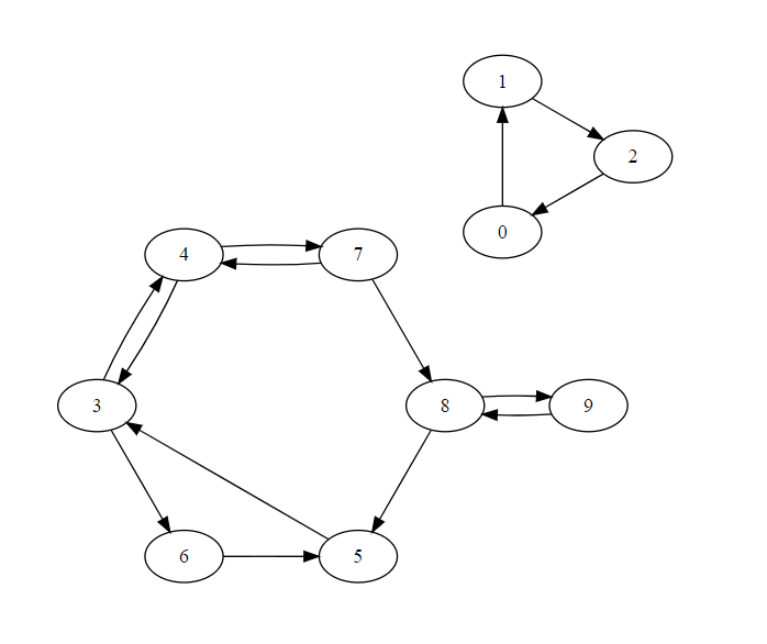
For given graph

Implementation of Find Connected Components in graph using BFS


x
1
# Queue Implementation
2
class Queue:
3
    def __init__(self):
4
        self.queue = []
5
    def enqueue(self,v):
6
        self.queue.append(v)
7
    def isempty(self):
8
        return(self.queue == [])
9
    def dequeue(self):
10
        v = None
11
        if not self.isempty():
12
            v = self.queue[0]
13
            self.queue = self.queue[1:]
14
        return(v)    
15
    def __str__(self):
16
        return(str(self.queue))
17

18
# BFS Implementation for Adjacency list
19
def BFSList(AList,start_vertex):
20
    visited = {}
21
    for each_vertex in AList.keys():
22
        visited[each_vertex] = False
23
    
24
    q = Queue()    
25
    visited[start_vertex] = True
26
    q.enqueue(start_vertex)
27
    
28
    while(not q.isempty()):
29
        curr_vertex = q.dequeue()
30
        for adj_vertex in AList[curr_vertex]:
31
            if (not visited[adj_vertex]):
32
                visited[adj_vertex] = True
33
                q.enqueue(adj_vertex)               
34
    return(visited)
35

36
# Implementation to find connected components in graph
37
def Components(AList):
38
    # Initialization of component value -1 for each vertex
39
    component = {}
40
    for each_vertex in AList.keys():
41
        component[each_vertex] = -1   
42
    
43
    # Initialize compid(represent conntected component id)
44
    # Initialize seen(represent number of visited/checked vertices)
45
    (compid,seen) = (0,0)
46
    
47
    # Repeat the following untill seen value is not equal to number of vertex
48
    while seen < max(AList.keys()):
49
        # Find the min level value vertex among all vertices which are not checked or visited
50
        startv = min([i for i in AList.keys() if component[i] == -1])
51
        # Call the BFS to check the reachability from startv
52
        visited = BFSList(AList,startv)  
53
        # Assign compid value to each reachable vertex from startv and increment seen value
54
        for vertex in visited.keys():
55
            if visited[vertex]:
56
                seen = seen + 1
57
                component[vertex] = compid
58
        
59
        # Increment compid by one to check again if any vertex are remaing to visisted 
60
        compid = compid + 1  
61
    
62
    return(component)
63

64

65
AList = {0: [1], 1: [2], 2: [0], 3: [4, 6], 4: [3, 7], 5: [3, 7], 6: [5], 7: [4, 8], 8: [5, 9], 9: [8]}
66
print(Components(AList))

Output


xxxxxxxxxx
1
1
{0: 0, 1: 0, 2: 0, 3: 1, 4: 1, 5: 1, 6: 1, 7: 1, 8: 1, 9: 1}

Pre and Post numbering using DFS

The Pre and Post numbering using DFS algorithm is used to assign a unique number to each node in a graph during a Depth-First Search (DFS) traversal.

Algorithm

Here are the steps for the Pre and Post numbering using DFS algorithm:

Initialize a counter count to 0 and two dictionary pre and post to keep track of the pre and post numbers of the nodes.
For each unvisited node u in the graph, perform a DFS traversal starting from u.
During the DFS traversal, visit each unvisited neighbor v of the current node u and recursively perform a DFS traversal starting from v.
Increment the count and assign it as the pre number of the current node u.
After all neighbors of the current node u have been visited, increment the count again and assign it as the post number of the current node u.
Repeat steps 3-5 until all nodes in the graph are visited.
Return the pre and post arrays.

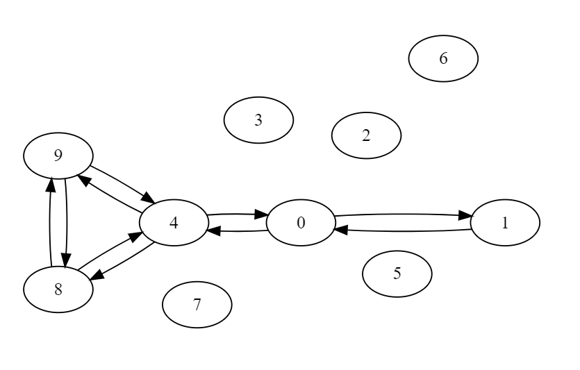
For given graph

Implementation of Pre and Post numbering on graph using DFS


xxxxxxxxxx
37
1
# Global variables
2
(visited,pre,post) = ({},{},{})
3

4
# Initialization
5
def DFSInitPrePost(AList):   
6
    for each_vertex in AList.keys():
7
        visited[each_vertex] = False
8
        (pre[each_vertex],post[each_vertex]) = (-1,-1)
9
    return
10

11
# Implementation of Pre and Post numbering on graph using DFS approch
12
def DFSListPrePost(AList,v,count):
13
    # Mark veretx v as visited
14
    visited[v] = True
15
    # Assigned the pre numbering for v when we are traversing the vertex(entering the vertex)
16
    pre[v] = count
17
    # Increment the count
18
    count = count + 1                      
19
    # Repeat for each unvisited adjacent of vertex v
20
    for adj_vertex in AList[v]:
21
        if (not visited[adj_vertex]):
22
            # Recursively call the DFSListPrePost on unvisited adjacent of v
23
            count = DFSListPrePost(AList,adj_vertex,count)
24
    # Assigned the post numbering for v when return back from recusrive call(leaving the vertex)
25
    post[v] = count
26
    # Increment the count
27
    count = count + 1                           
28
    
29
    return(count)
30

31

32
AList = {0: [1, 4],1: [0],2: [],3: [],4: [0, 8, 9],5: [],6: [],7: [],8: [4, 9],9: [8, 4]}
33
DFSInitPrePost(AList)
34
print(DFSListPrePost(AList,0,0))
35
print(visited)
36
print(pre)
37
print(post)

Output


xxxxxxxxxx
4
1
10
2
{0: True, 1: True, 2: False, 3: False, 4: True, 5: False, 6: False, 7: False, 8: True, 9: True}
3
{0: 0, 1: 1, 2: -1, 3: -1, 4: 3, 5: -1, 6: -1, 7: -1, 8: 4, 9: 5}
4
{0: 9, 1: 2, 2: -1, 3: -1, 4: 8, 5: -1, 6: -1, 7: -1, 8: 7, 9: 6}

Classifying tree edges in directed graphs using pre and post numbering

Tree edge/forward edge:

Edge (u, v) is tree/forward edge, if Interval [pre(u), post(u)] contains [pre(v), post(v)]

Back edge:

Edge (u, v) is back edge, if Interval [pre(v), post(v)] contains [pre(u), post(u)]

Back edges generate cycles

Cross edge:

Edge (u, v) is cross edge, if Intervals [pre(u), post(u)] and [pre(v), post(v)] are disjoint

Directed Acyclic Graph(DAG)

A Directed Acyclic Graph(DAG) is a directed graph with no directed cycles. That is, it consists of vertices and edges, with each edge directed from one vertex to another, such that following those directions will never form a closed loop.

Directed acyclic graphs are a natural way to represent dependencies

Arise in many contexts
- Pre-requisites between courses for completing a degree
- Recipe for cooking
- Construction project
Problems to be solved on DAG
- Topological sorting
- Longest paths

Topological Sort

The Topological Sort algorithm is used to sort the nodes of a directed acyclic graph (DAG) in such a way that for every directed edge from node u to node v, node u comes before node v in the sorting order.

Algorithm

Here are the steps for the Topological Sort algorithm:

Compute the in-degree of each node in the graph.
Enqueue all nodes with in-degree 0 to a queue.
While the queue is not empty, dequeue a node from the front of the queue and add it to the sorted list.
For each of the dequeued node's neighbors, decrement their in-degree by 1.
If any of the dequeued node's neighbors now have in-degree 0, enqueue them to the queue.
Repeat steps 3-5 until the queue is empty.

If the graph contains a cycle, the Topological Sort algorithm cannot produce a valid sorting order because it is impossible to order the nodes such that all edges point forward. In this case, the algorithm will terminate with an error or produce an incomplete sorting order.

To keep track of the sorting order, you can add each dequeued node to a list as it is dequeued from the queue.

$O(V^2 )$ $O(V + E)$ $V$ $E$ is number of edges in Graph.

Working Visualization

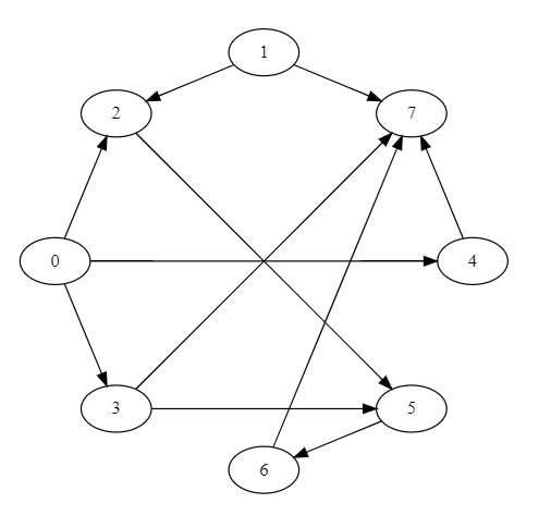
For given graph(DAG)

Implementation of Topological Sort for Adjacency list


xxxxxxxxxx
55
1
# Implementaion of Queue
2
class Queue:
3
    def __init__(self):
4
        self.queue = []
5
    def enqueue(self,v):
6
        self.queue.append(v)
7
    def isempty(self):
8
        return(self.queue == [])
9
    def dequeue(self):
10
        v = None
11
        if not self.isempty():
12
            v = self.queue[0]
13
            self.queue = self.queue[1:]
14
        return(v)    
15
    def __str__(self):
16
        return(str(self.queue))
17

18
# Implementation of Topological sort for Adjacency list
19
def toposortlist(AList):
20
    # Initialization
21
    (indegree,toposortlist) = ({},[])
22
    zerodegreeq = Queue()
23
    for u in AList.keys():
24
        indegree[u] = 0
25
    
26
    # Compute indegree for each vertex
27
    for u in AList.keys():
28
        for v in AList[u]:
29
            indegree[v] = indegree[v] + 1
30
    
31
    # Find the vertex with indegree 0 and added into the queue
32
    for u in AList.keys():
33
        if indegree[u] == 0:
34
            zerodegreeq.enqueue(u)
35
    
36
    # Topological sort Computing process
37
    while (not zerodegreeq.isempty()):
38
        # Remove one vertex from queue which have zero degree vertices
39
        curr_vertex = zerodegreeq.dequeue()       
40
        # Store the removed vertex in toposortlist and reduce the indegree by one 
41
        toposortlist.append(curr_vertex)
42
        indegree[curr_vertex] = indegree[curr_vertex]-1
43
        
44
        # Repeat for each adjacent of the removed vertex
45
        for adj_vertex in AList[curr_vertex]:
46
            # Reduce the indegree of each adjacent of the removed vertex by 1
47
            indegree[adj_vertex] = indegree[adj_vertex] - 1
48
            # If after reducing the degree of adjacent, it becomes zero then insert it into the queue
49
            if indegree[adj_vertex] == 0:
50
                zerodegreeq.enqueue(adj_vertex)                
51
    
52
    return(toposortlist)
53

54
AList={0: [2, 3, 4], 1: [2, 7], 2: [5], 3: [5, 7], 4: [7], 5: [6], 6: [7], 7: []}
55
print(toposortlist(AList))

Output


xxxxxxxxxx
1
1
[0, 1, 3, 4, 2, 5, 6, 7]

Code Execution Flow

Implementation of Topological Sort for Adjacency matrix


xxxxxxxxxx
37
1
# Implementation of Topological sort for Adjacency matrix
2
def toposort(AMat):
3
    #Initialization
4
    (rows,cols) = AMat.shape
5
    indegree = {}
6
    toposortlist = []
7
    
8
    #Compute indegree for each vertex
9
    for c in range(cols):
10
        indegree[c] = 0
11
        for r in range(rows):
12
            if AMat[r,c] == 1:
13
                indegree[c] = indegree[c] + 1
14
    
15
    # Topological sort Computing process
16
    for i in range(rows):
17
        # Select the min level vertex for removing the graph which has indegree 0
18
        j = min([k for k in range(cols) if indegree[k] == 0])
19
        # Store the removed vertex j in toposortlist and reduce the indegree by one 
20
        toposortlist.append(j)
21
        indegree[j] = indegree[j] - 1
22
        
23
        # Reduce the indegree of each adjacent of the removed vertex j by 1
24
        for k in range(cols):
25
            if AMat[j,k] == 1:
26
                indegree[k] = indegree[k] - 1
27
                
28
    return(toposortlist)
29

30

31
edges=[(0,2),(0,3),(0,4),(1,2),(1,7),(2,5),(3,5),(3,7),(4,7),(5,6),(6,7)]
32
size = 8
33
import numpy as np
34
AMat = np.zeros(shape=(size,size))
35
for (i,j) in edges:
36
    AMat[i,j] = 1
37
print(toposort(AMat))

Output


xxxxxxxxxx
1
1
[0, 1, 2, 3, 4, 5, 6, 7]

Longest Path in DAG

The Longest Path in an unweighted Directed Acyclic Graph (DAG) algorithm is used to find the maximum length path in a DAG.

Algorithm

Here are the steps for the Longest Path in an Unweighted DAG algorithm:

Topologically sort the nodes in the graph using the Topological Sort algorithm.
Initialize a distance array with all nodes set to 0 except the source node, which is set to 0.
For each node u in the topologically sorted order, iterate through its incoming edges (v, u) and update the distance of node u as max(dist[u], dist[v] + 1).
The longest path length will be the maximum value in the distance array.

$O(V + E)$ $V$ $E$ is number of edges in Graph.

Working Visualization

For given graph(DAG)

Implementation for Longest Path on DAG


xxxxxxxxxx
56
1
# Implementation of Queue
2
class Queue:
3
    def __init__(self):
4
        self.queue = []
5
    def enqueue(self,v):
6
        self.queue.append(v)
7
    def isempty(self):
8
        return(self.queue == [])
9
    def dequeue(self):
10
        v = None
11
        if not self.isempty():
12
            v = self.queue[0]
13
            self.queue = self.queue[1:]
14
        return(v)    
15
    def __str__(self):
16
        return(str(self.queue))
17

18
# Implementation Longest path on DAG for Adjacency list
19
def longestpathlist(AList):
20
    # Initialization
21
    (indegree,lpath) = ({},{})
22
    zerodegreeq = Queue()
23
    for u in AList.keys():
24
        (indegree[u],lpath[u]) = (0,0)
25
    
26
    # Compute indegree for each vertex
27
    for u in AList.keys():
28
        for v in AList[u]:
29
            indegree[v] = indegree[v] + 1
30

31
    # Find the vertex with indegree 0 and added into the queue
32
    for u in AList.keys():
33
        if indegree[u] == 0:
34
            zerodegreeq.enqueue(u)
35
            
36
    # Longest path computing process            
37
    while (not zerodegreeq.isempty()):
38
        # Remove one vertex from queue which have zero degree vertices and reduce the indegree by 1
39
        curr_vertex = zerodegreeq.dequeue()
40
        indegree[curr_vertex] = indegree[curr_vertex] - 1
41
        
42
        # Repeat for each adjacent of the removed vertex 
43
        for adj_vertex in AList[curr_vertex]:
44
            # Reduce the indegree of each adjacent of the removed vertex by 1
45
            indegree[adj_vertex] = indegree[adj_vertex] - 1
46
            # Assign the longest path value for each adjacent of the removed vertex
47
            lpath[adj_vertex] = max(lpath[adj_vertex],lpath[curr_vertex]+1)
48
            # If after reducing the degree of adjacent, it becomes zero then insert it into the queue
49
            if indegree[adj_vertex] == 0:
50
                zerodegreeq.enqueue(adj_vertex)
51
                
52
    return(lpath)
53

54

55
AList={0: [2, 3, 4], 1: [2, 7], 2: [5], 3: [5, 7], 4: [7], 5: [6], 6: [7], 7: []}
56
print(longestpathlist(AList))

Output


xxxxxxxxxx
1
1
{0: 0, 1: 0, 2: 1, 3: 1, 4: 1, 5: 2, 6: 3, 7: 4}

Code Execution Flow

Visualization of graph algorithms using visualgo

Select the BFS/DFS/Topological sort algorithm from left menu to visualize the working.

Source - https://visualgo.net/en/dfsbfs